By Class of Winter Term 2017 / 2018 | December 14, 2017
TEST
#hugo
import numpy as np
import pandas as pd
2+3
A Gentle Introduction to Neural Network Fundamentals
#### Imagine the following problem:
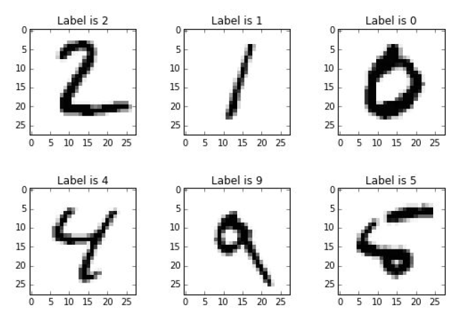
There are handwritten numbers that you want computer to correctly clasify. It would be an easy task for a person but an extremely complicated one for a machine, especially, if you want to use some traditional prediction model, like linear regression. Even though the computer is faster than the human brain in numeric computations, the brain far outperforms the computer in some tasks.
Source: https://www.jstor.org/stable/pdf/2684922.pdf
Some intuition from the Nature
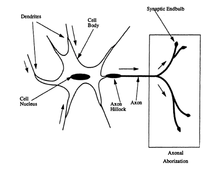
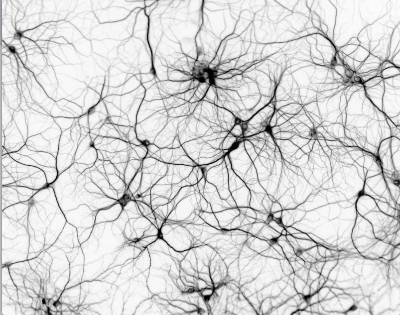
People struggled to teach machines to solve this kind of problems for a long time without success. Unless they noticed a very peculiar thing. Nature creatures, even the simple ones, for instance insects, can perform complicated task with very limited brain capacities, which are far below those of the computers. So there is something nature has developed that aloows to solve tasks apparently complicated for machines tasks in a smart way. One of the ides that came to mind is to replicate the structure and certain functions of nature beigns brain and neurosystem that allow for cognitive procecess and beyond. A particular example of such structures is neuron system.
[Source: https://www.jstor.org/stable/pdf/2684922.pdf]
[Source: https://pixabay.com/]
A particular detail about how are our cognitive and perceptive processes organised is a complicated structure of simple elements which create a complex net where each element is connected with othere receiving and transmitting information. An idea to reemplement such a structure in order to make predictions gave birth to what we now now as neural network models.
Early development:
1943
McCulloch-Pitts model of the neuron. The neuron receives a weighted sum of inputs from connected units, and outputs a value of one (fires) if this sum is greater than a thresh- old. If the sum is less than the threshold, the model neuron outputs a zero value.
Early 1960s
Rosenblatt developed a model called simple perceptron. The simple perceptron consists of McCulloch- Pitts model neurons that form two layers, input and output. His model was able to find a solution to classification problems if the problem was linearly separable. Later on Minsky and Papert addressed the linear severability limitation of Rosenblatt model. He knew it himself but could not figure it out. This hindered the process of NNs development.
1982
Hopfield Model used mainly for optimization problems like travel sales man problem Later on, the idea of backpropagation was introduced and it addressed the earlier problems of the simple perceptron and renewed interest in neural networks. Backpropagation training algorithm is capable of solving nonlinear separable problems.
Differnt Applications
At the current stage NNs are capable to model many of the capabilities of the human brain and beyond. On a practical level the human brain has many features that are desirable in an electronic computer. The human brain has the ability to generalize from abstract ideas, recognize patterns in the presence of noise, quickly recall memories, and withstand localized damage.
Usages of NNS:
- identifying underwater sonar contacts
- predicting heart problems in patients
- diagnosing hypertension
- recognizing speech
- the preferred tool in predicting protein secondary structures
Staticians use these models to address the same problems:
- discriminant analysis
- logistic regression
- Bayes and other types of classifiers
- multiple regression
- time series models such as ARIMA and other forecasting methods
Schematic Representation
All the aplications of neural networks mentioned above have in common a simlified structure depicted on the following picture.
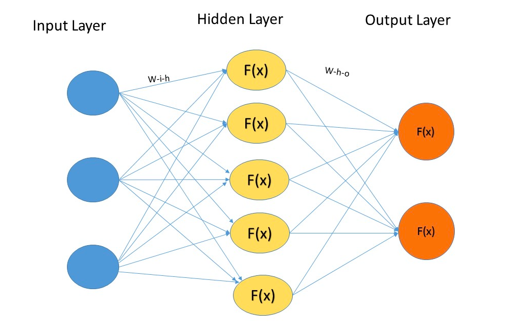
### Implementation of the NN from scratch Let's try to reimlement such a structure using Python. The crutial elements are:
- layers
- nodes
- weights between them
- activation function
Activation Function
Besides complicated multilayer structure with many nodes neurosystems in nature has one more important feature - neurons in them send signal further or "fire" only when they get a signal that is strong enough - stronger than certain treshold. This can be represented by a step function.
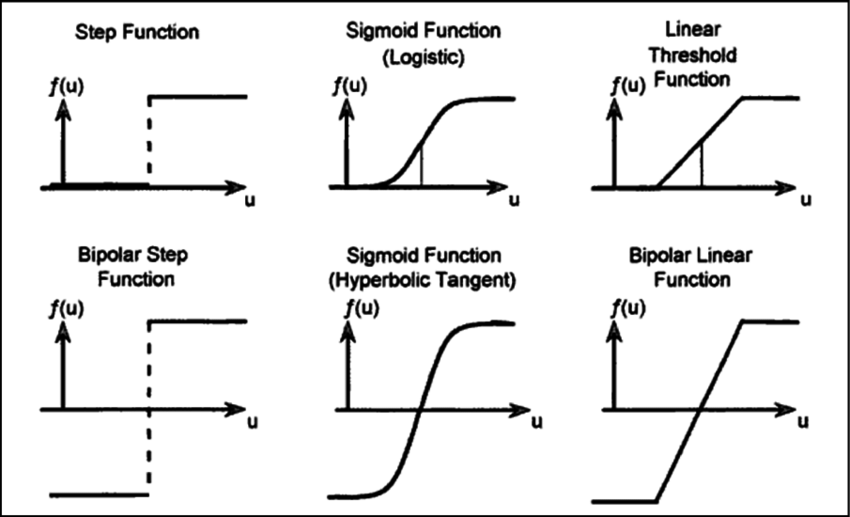
[Source:https://www.researchgate.net/figure/Three-different-types-of-transfer-function-step-sigmoid-and-linear-in-unipolar-and_306323136]
Inspect the Data
It seems like all the elements of our neural network structure are ready. Can we use this structure to tackle the problem?
Let’s take a look at our data.
### Fit draft of the NN to the Data
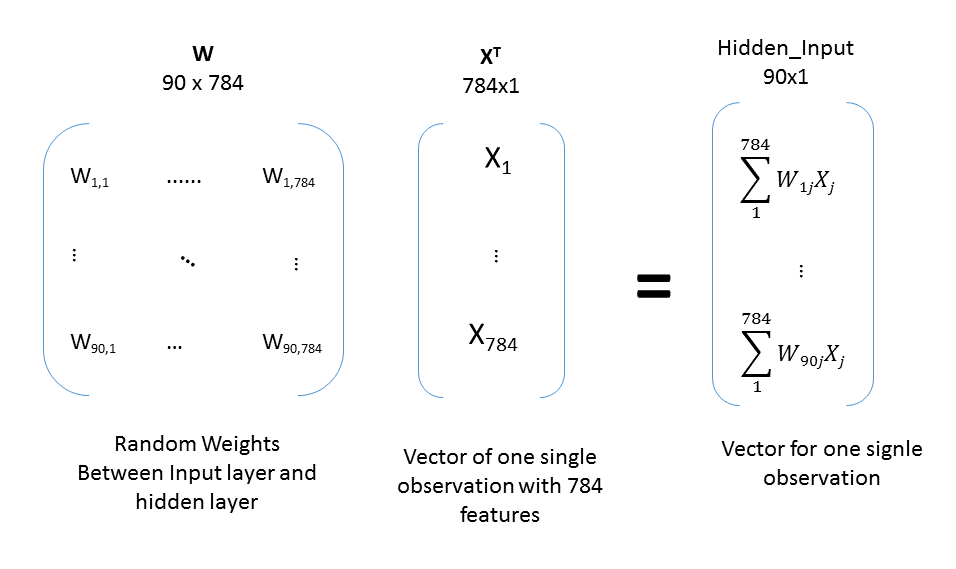
As we can see we have 784 elements in our inputs. Therefore it would be logical to update the structure of the neural network. Instead of 3 input nodes we will have 784. Accordinly, as we have 10 different options for the outcome *from 0 to 9) we schould better have 10 output nodes instead of 1. 100 nodes in the hidden layer have been assigned as something in between 784 and 10.
Feed forward
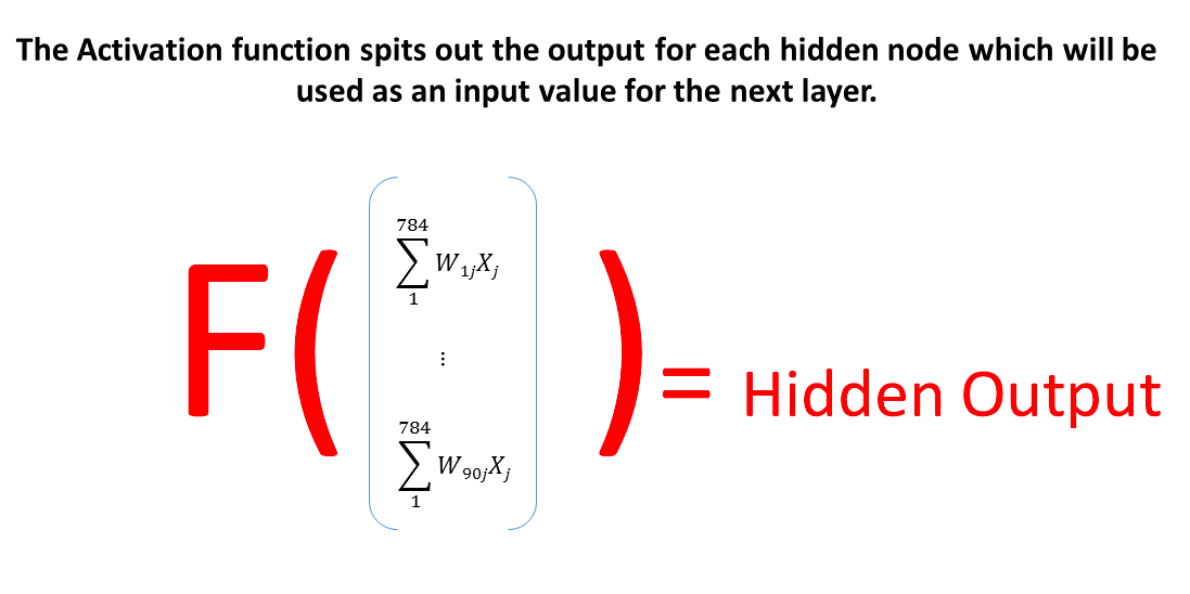
Once we have the structure of the NN updated for the specific task of prediciting numbers depicted on the images, we can run our network to get its first predictions. To do so we will have to make several steps and each of them will consist of a matrix multiplication and application of the sygmoid function. Multiply a vector of inputs by a matrix of weights that connects it with the next layer, transform the result using activation function - this is one step and it schould be repeated for all the layers except for the input one. Every time the output of the previous leyer will be used as a vector of inputs for the next layer.
- It seems like we have some serious mistake here.
- Already at the point of h_outputs all the data converts to 1.
- There could be several reasons for that.
- First of all, let’s take a look at our sigmoid function once again:
Why don’t we get what we expected?
### How good are we now? ### Backpropagation Output of each node is the sum of the multiplications of the outputs of previous nodes by certain weights. Therefore we can associate how much error is comming with every weight and how much error has been brought from each particular node from the previous layer as depicted on the pictures below.