By Seminar Information Systems (WS19/20) | February 7, 2020
Economic Uncertainty Identification Using Transformers - Improving Current Methods
Authors: Siddharth Godbole, Karolina Grubinska & Olivia Kelnreiter

Table of Contents
- Introduction
- Motivation and Literature
- Theoretical Background
3.1 Transformers, BERT and BERT-based Models
3.2 Transformers Architecture
3.3 BERT
3.4 RoBERTa
3.5 DistilBERT
3.6 ALBERT
3.7 Comparing RoBERTa, DistilBERT and ALBERT - Application to Economic Policy Uncertainty
4.1 Data Exploration
4.1.1 Data Pre-Processing
4.1.2 Data Imbalance
4.2 Models Implementation
4.2.1 Transformer-Based Models
4.2.2 Benchmarks
4.2.3 Interpretation of Results - Further Discussion
5.1 Optimal Threshold Calculation
5.2 Impact of Certain Tokens in Identifying Uncertainty - Conclusions
- References
1. Introduction
Within the past week, Brexit happened. The U.S. primaries for the next presidential election started. Donald Trump continues to fight for reelection while being acquitted in an impeachment trial. From events like these, economic policy uncertainty rises and households and firms take actions with wider impacts. To better analyze and predict these sentiments of economic policy uncertainty, Baker et al. (2016) built an economic policy uncertainty index. They analyzed whether newspaper articles contained references to economic policy uncertainty - but did so with a relatively simple search term and 12,000 human-labeled articles. Recently, much more complex classification algorithms have emerged in natural language processing (NLP). Researchers in the field are developing new and better language models at an unprecedented speed (Sanh 2019a). Applying these new state of the art models could improve current methods and replace manual labeling tasks for indices such as the economic policy uncertainty index, but also find widespread application in business and other fields. In this project, we want to test this: we apply new transformer models from the BERT-family to improve the current method of binary text classification in the context of economic policy uncertainty. We find that all of our models achieve remarkable results in classifying the given newspaper data (AUC’s ranging from 0.87-0.90), with RoBERTa achieving the best results compared to BERT, DistilBERT, and ALBERT (as well as the non-transformer benchmarks). This indicates that the models are well equipped to take over tasks that researchers have previously solved in less optimal ways. To illustrate this finding, this blog post is organized as follows: in section 2. Motivation and Literature we give context on the case study of economic policy uncertainty, followed by 3. Theoretical Background where we present and explain how transformers and specifically the four states of the art BERT-models work. In 4. Application to Economic Policy Uncertainty, we demonstrate the implementation of the BERT-models to our case study and present the results. Finally, we highlight important considerations and take-aways in section 5. Further Discussion.
2. Motivation and Literature
Economic policy uncertainty can have substantial effects on the decisions of individual economic actors, like firms or households. “Uncertainty is the No 1 enemy of investment markets”, as Huang (2019) put it. To facilitate research on the topic, Baker et al. (2016) developed their Economic Policy Uncertainty (EPU) index. Initially, their analysis was conducted for the United States, but they and other researchers have since extended the methodology to other world markets. Currently, the EPU analyses on their website can be viewed for 25 countries as well as on a global level. The index is a good case study for applying state of the art NLP models, because the application of such models could improve their methodology and replace human labeling.
The EPU index stems from analyzing different newspaper articles and the coverage of topics related to economic uncertainty. In the original methodology, Baker et al. searched 10 major U.S. newspapers from 1985 - 2013 in the papers’ digital archives for the keywords “economic” or “economy”, “policy” and “uncertain” or “uncertainty”. If an article contains all three keywords (and at least one from a list of words related to policy), it is marked as “1” (= it contains economic policy uncertainty). Based on the monthly frequency (accounting for the overall volume of articles in that time span), they create the EPU index. Various different keywords could be included here for customized analyses (which Baker et al. also do for several different policy fields). For example, if a Brexit related EPU index is to be calculated then “brexit” as a keyword could be included and then analyzed. Below is an example of the EPU index for the UK, comparing overall and Brexit-related economic policy uncertainty. The graph, taken from Baker et al.‘s website, allows us to analyze trends and major changes during that time.
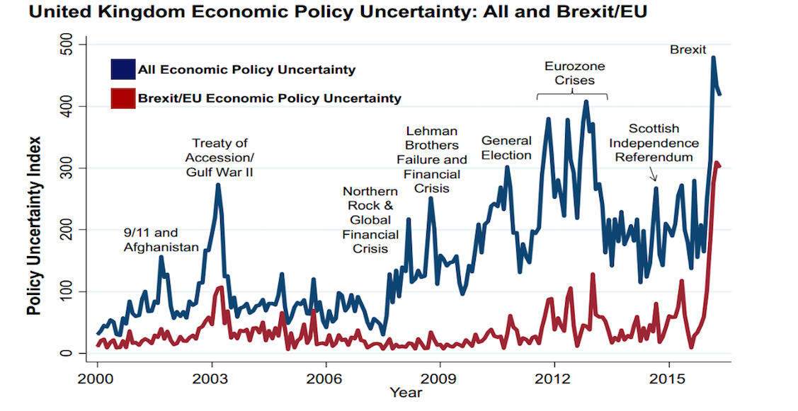
Brexit and Policy Uncertainty. From What is Brexit-Related Uncertainty Doing to United Kingdom Growth? 2016. http://www.policyuncertainty.com/brexit.html.
Baker et al. (2016)‘s approach also involved a human audit study: over an 18-month-period, student-teams manually classified over 12,000 articles for economic policy uncertainty. However, this is a tedious task and such an audit study is not easily replicable. With recent advances in the field of NLP in mind, we want to expand this methodology beyond the simple identification of keywords, and replace human classification by reliable, automated methods.
3. Theoretical Background
In order to use the best methods possible to identify economic uncertainty in the newspaper articles, we decided to apply BERT-based transformers. In a very short time, transformers and specifically BERT have literally transformed the NLP landscape with high performance on a wide variety of tasks. New, improved models are published every few weeks (if not days) and much remains to be researched and developed further. An example of the ongoing scientific discussions in the field is the trend to build ever larger and heavier models to improve performance. The image below shows this trend by plotting selected models by publishing date and parameter size. But do more parameters always increase a model’s performance? What are other ways of improving models? To answer these and other questions, we devote this chapter to laying the theoretical groundwork: we will explain the basic transformer architecture and BERT, and then present three models (RoBERTa, DistilBERT, ALBERT) that promise to outperform BERT on different dimensions, before applying them to our binary text classification task in the next chapter.
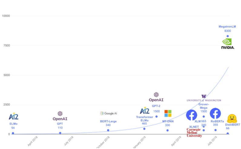
Evolution of Transformer-Based Models. Created by Victor Sanh. 2019. From ,,Smaller, Faster, Cheaper, Lighter: Introducing DilstilBERT, a Distilled Version of BERT.’’ Medium (blog). https://medium.com/huggingface/distilbert-8cf3380435b5
3.1 Transformers, BERT and BERT-based Models
Highly complex convolutional and recurrent neural networks (CNNs and RNNs) achieved the best results in language modeling tasks, before Vaswani et al. (2017) proposed a simpler network architecture. The advantages of this newly born transformer were threefold: (1) it allowed for a parallelization of tasks, (2) resulted in simpler operations, and (3) achieved better results overall. How did Vaswani et al. do this? Their idea was to build a model based on attention mechanisms, which some of the CNNs and RNNs at that time used to connect their encoder and decoder. As the BERT family is built on the transformer architecture and it is helpful to have a basic understanding of it, we devote a short subchapter to the attention-based architecture. For a more in-depth explanation, we recommend taking a look at Jay Alammar’s Illustrated Transformer or Harvard NLP’s Annotated Transformer.
3.2 Transformers Architecture
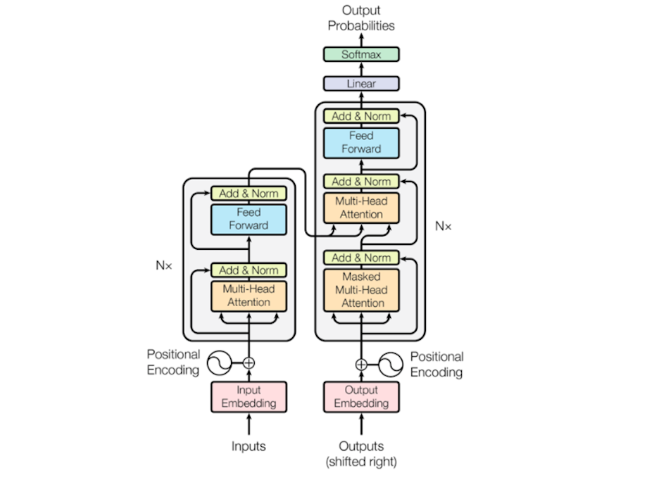
Transformers Architecture. Created by Vaswani et al. 2017. From ,,Attention is All You Need.’’ http://arxiv.org/abs/1706.03762
Adapted from Vaswani et al., the figure above displays a transformer. On the left side is the encoder, next to it on the right the decoder. As in preceding models, the encoder is responsible for forming continuous representations of an input sequence. The decoder in turn maps these representations back to output sequences. Both encoder and decoder consist of several layers (denoted with Nx in the graph) with two and three sub-layers each, respectively:
-
Multi-Head Attention: here, keys, values and queries (which come from the self-attention - in this case, the previous layer’s output) are linearly projected to then perform the attention function in parallel (which Vaswani et al. call the “scaled dot-product attention”). The multi-head characteristic makes it possible to use “different representation subspaces at different positions” (Vaswani et al., 4).
-
Masked Multi-Head Attention (only in decoder): as the first sub-layer in the decoder, this layer performs the multi-head attention on the encoder’s output. It is masked in order to prevent predictions based on information that must not be known yet at a certain position.
-
Feed Forward Network: two linear transformations are applied to each position separately and identically.
Before information enters the layers, the positional encoding conveys information on the relative position of a token in a sequence and allows the transformer to make use of the token order. Once the layers have performed their attention function and transformations, another two transformations take place: the Linear, applying another linear transformation, and the Softmax, which transforms the output back to probabilities.
3.3 BERT
BERT (Bidirectional Encoder Representations from Transformers) was published in 2018 by Devlin et al. from Google and performed so well that - within a year - it inspired a whole model-family to develop. BERT built on the original transformer idea, but used a slightly changed architecture, different training, and (as a result) increased size.
-
Architecture: BERT’s architecture is largely based on the original transformer but is larger (even in its base version) with more layers, larger feed-forward networks and more attention heads.
-
Training: The real innovation comes in the bidirectional training that BERT performs. There are two pre-training tasks: masked language modeling (MLM) and next sentence prediction (NSP). These are performed on the pre-training data of the BookCorpus (800 million words) and English Wikipedia (2500 million words).
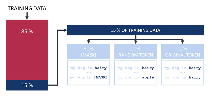
- Masked Language Modeling (MLM): to train the model bidirectionally, Devlin et al. (2018) let BERT predict masked words based on the context. They randomly hide 15% of the tokens in each sequence. Of these 15% of tokens, however, only 80% are replaced with a [MASK] token, 10% are replaced with a random other token, and 10% are unchanged.
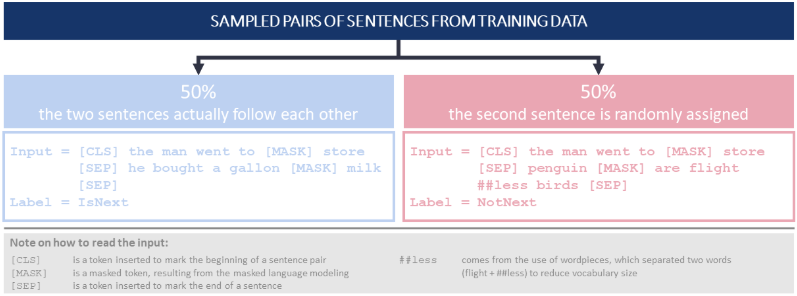
- Next Sentence Prediction (NSP): To also train the model on the relationship between sentences, Devlin et al. (2018) decided to apply a NSP task. BERT has to decide for pairs of sentence segments (each segment can consist of several sentences) whether they actually succeed each other or not (with a 50% probability of either case being true).
- Size: Overall, the changes result in a larger model with 110 million parameters in the case of BERT-Base and 340 million parameters for BERT-Large.
As mentioned, when published, BERT dominated performance benchmarks and thereby inspired many other authors to experiment with it and publish similar models. This led to the development of a whole BERT-family, each member being specialized on a different task. Take for example SpanBERT which aims to improve pre-training by representing and predicting spans or CamemBERT, a French-language BERT. We chose to apply three particularly prominent BERT-based models, RoBERTa, DistilBERT and ALBERT, each of which was developed with a different goal in mind and brought new insights to the world of NLP models.
Check out the graph below to get an overview of the many BERT-models and their publishing date (not exhaustive!).
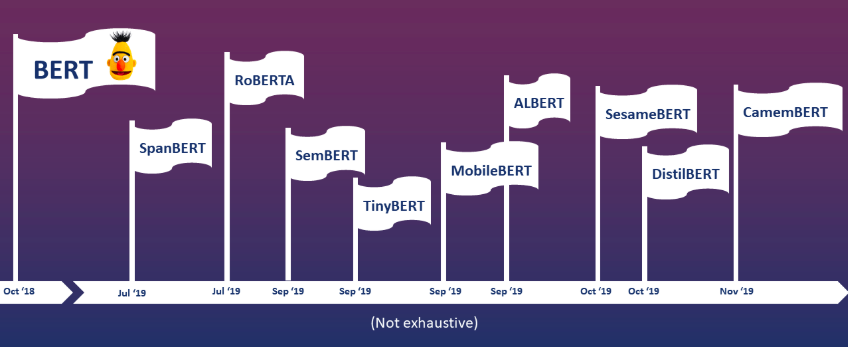
The Bert Family
3.4 RoBERTa
One of the first to follow BERT’s architecture were Liu et al. (2019), a team of researchers from Facebook AI. In July 2019, they published a model called RoBERTa (which stands for Robustly-optimized BERT approach). The authors saw room for improvement in the pre-training, arguing that BERT was significantly undertrained. They changed some pre-training configurations, and RoBERTa outperformed BERT on the GLUE benchmark.
Since RoBERTa was developed based on BERT, the two models share the transformer architecture. However, Liu et al. examined some of BERT’s pre-training settings in an experimental setup and subsequently decided to implement the following changes:
-
Additional Training Data: As mentioned before, BERT was trained on the BookCorpus and English Wikipedia with the overall size of 16 GB. For RoBERTa, Liu et al. used those two datasets and on top of it three additional sources:
-
CC-News: collected by the authors from the English portion of the CommonCrawl News dataset in the time period between September 2016 and February 2019. (76GB)
-
Stories: a dataset containing a subset of CommonCrawl data filtered to match the story-like style of Winograd schemas. (31GB)
-
OpenWebText: a web content extracted from URLs shared on Reddit with at least three upvotes. (38GB)
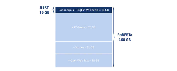
In total, the data used to train RoBERTa was a huge English-language uncompressed text corpus 10 times larger than what BERT was trained on: 160 GB of text.
- Dynamic Masking Pattern: BERT’s masking approach relied on performing masking once during data pre-processing, which resulted in one static mask. Liu et al. adjusted this method when trying different versions of masking for RoBERTa: first, they duplicated the data 10 times over 40 epochs of training. This resulted in four masks, where each training sequence was seen only four times during training procedure (once per mask) instead of every time within one mask. Then, the authors also compared this approach with dynamic masking, where the mask is generated every time the sequence is passed to the model.
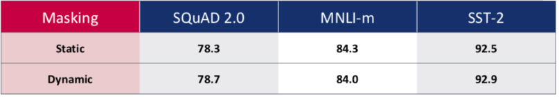
As shown above, the dynamic masking provided some improvements in performance. The authors also mentioned that using it resulted in efficiency benefits and therefore, they decided to train RoBERTa using the dynamic masking approach.
-
Removing the Next Sentence Prediction Objective (NSP): Another significant change compared to the original BERT emerged from experimenting with the Next Sentence Prediction objective during the training of a model. Predicting if two segments of text appear together (as in case of BERT) was meant to train the model in capturing the relationships between sentences and learning its context. Liu et al. compared the performance of RoBERTA in four different settings:
- The segment pair approach is the original BERT setting trained with NSP loss, where the model takes a pair of segments as input and has to predict if these two appear together. One segment can contain multiple natural sentences (until it reaches 512 tokens).
- The sentence-pair approach is similar to what was originally implemented in BERT, with the difference that instead of segments (which can contain multiple sentences), every pair really consists only of two sentences on which the NSP is applied.
- In the full-sentences case, the training input are full sentences coming from one or more documents. When the input reaches the end of one document it will start sampling from another one (until it reaches 512 tokens).The authors removed the NSP loss from the training objective.
- doc-sentences work in the same way as full-sentences, with the difference that the inputs may only come from one document. In this case, the length of tokens may be shorter than 512 tokens. Therefore, the authors decided to increase the batch size in order to achieve a similar number of tokens to the previous cases. Again, there is no training on NSP loss.
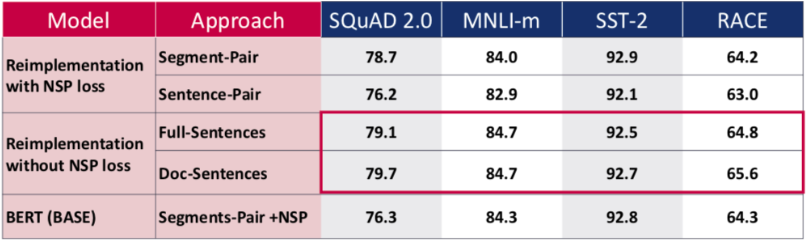
As can be seen in the table above, the new settings outperformed the originally published BERT (BASE) results. Removing the NSP loss led to improvements while testing on four different tasks. Doc-Sentences performed best, but resulted in an increased batch size and less comparability - therefore, Liu et al. decided to use Full-Sentences in the remainder of their experiments.
- Training with Larger Batches: The original BERT (BASE) was trained over 1 million steps with a batch size of 256 sequences. Liu et al. note that training over fewer steps with an increased batch size would be equivalent in terms of computational costs. Experimenting with those settings, they find out that training with bigger batches over fewer steps can indeed improve perplexity for the masked language modeling pattern and also the final accuracy.
3.5 DistilBERT
An ongoing trend in NLP and the further development of the BERT family has been to create ever heavier and larger models to improve performance (such as RoBERTa). BERT is costly, time-consuming and computationally heavy. Therefore, Sanh et al. (2019) from the NLP company Hugging Face researched how to improve BERT on these aspects while keeping performance high. In the end, they built a distilled version of BERT, which they called DistilBERT.
With DistilBERT, Sanh et al. showed that it is possible to reach and achieve 97% of BERT’s language understanding capabilities, while reducing the size of BERT model by 40%. Moreover, this model is 60% faster. While relying on the BERT architecture and using the same training data, DistilBERT implemented some ideas from RoBERTa and used a knowledge distillation process for the training of the model.
-
Architecture: DistilBERT has the same transformer architecture as BERT, but a smaller number of layers in order to reduce the model size. Sanh et al. also removed the token-type embeddings and pooler (which BERT uses for the next sentence classification task).
-
Training & Knowledge Distillation:
-
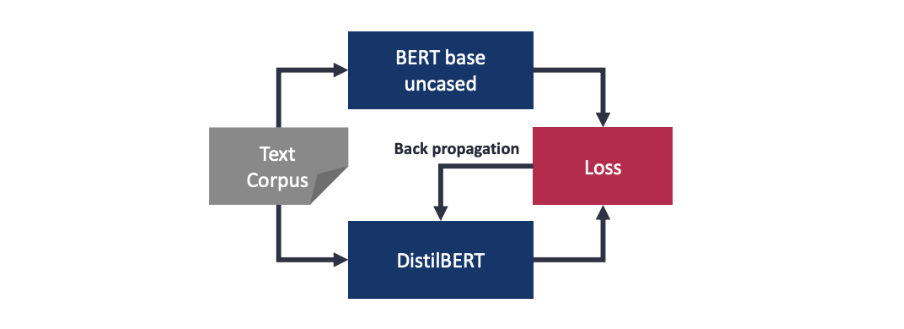
Knowledge Distillation: The name “DistilBERT” is derived from the distillation process, often seen in scientific applications such as separating water and salt. In the context of NLP, distillation refers to knowledge distillation which means to train a student model (DistilBERT) based on an already trained teacher model (BERT). In this case, DistilBERT is trained to replicate the behavior of BERT by matching the output distribution - training through knowledge transfer, so to say. The graph below provides a schematic overview of the DistilBERT training (technically simplified).
-
Training losses: Sanh et al. use three training losses for DistilBERT: distillation loss, masked language modeling loss (from the MLM training task) and cosine embedding loss (to align the directions of the student and teacher hidden states vectors). Triple losses ensure the student model learns properly and has efficient transfer of knowledge.
-
Batch size and next-sentence prediction: Building on what Liu et al. (2019) found for RoBERTa, Sanh et al. removed the NSP task for model training. They also changed the batch size from the original BERT to further increase performance (see “Training with Larger Batches” in the previous chapter).
For a more in-depth explanation, also take a look at Sanh’s blogpost on DistilBERT!
3.6 ALBERT
Whereas RoBERTa focused on performance and DistilBERT on speed, ALBERT (A Lite BERT) is built to address both. Lan et al. (2019) from Google in their paper achieve better results with lower memory consumption and increased training speed compared to BERT. They claim that BERT is parameter inefficient and apply techniques to reduce the parameters to 1/10th of the original model without substantial performance loss. Building on the BERT architecture, the authors experiment with two methods to reduce the model size: factorized embedding parameterization and cross-layer parameter sharing. In addition, they improve the model training by changing the next-sentence-prediction task for sentence-order-prediction. They keep the same training data as BERT and DistilBERT.
-
Factorized Embedding Parameterization (Architecture): In BERT and subsequent models, the size of WordPiece embeddings and the size of the hidden layers is linked. Lan et al. argue that this is inefficient, because each of the two has a different purpose. WordPiece embeddings supposedly capture the general meanings of words, which is context independent, whereas hidden layers map the meaning dependent on the specific context. Hidden layers therefore are much more complex: they need to store more information and be updated more often during the training process. In ALBERT, Lan et al. decompose the large vocabulary matrix into two smaller matrices. Thereby, they separate the size of the layers and reduce the number of model parameters significantly.
-
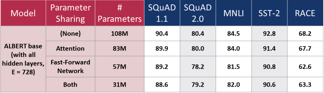
Cross-Layer Parameter Sharing (Architecture): Another way to reduce parameter size is by parameter sharing across layers. Lan et al. try three different settings for parameter sharing: sharing the feed-forward network parameters, the attention parameters, and sharing both at the same time. Parameter sharing prevents the number of parameter to grow with the depth of the network. However, there is a payoff between the model size and its performance. The table below (adapted from Lan et al.) shows: the ALBERT model with no parameter sharing has the largest size of parameters and best performance across NLP benchmarks. As the number of parameters decreases (with increasing sharing of parameters), performance also decreases. Lan et al. prefer the gain in efficiency over the highest performance. Therefore, they decide to share parameters across both as a default.
-
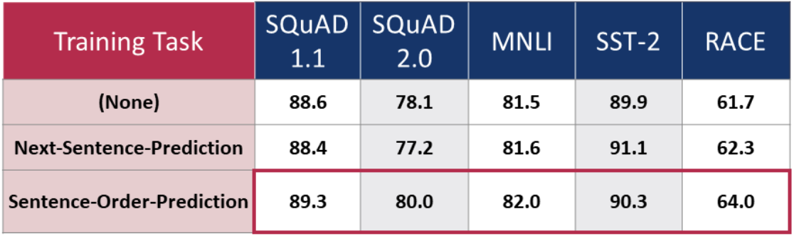
Sentence Order Prediction (Training) (SOP): The authors of RoBERTa have already shown that BERT’s NSP might not be the best training task. Lan et al. have a hypothesis why this is the case: NSP aims to teach the model coherence prediction. However, whether two sentences succeed each other can also be predicted from their topics - which for the model is easier to learn and overlaps with the MLM task. Learning to decide whether sentences belong together based on their topics, therefore does not add predictive power. Lan et al. find another coherence training task, which is more different from what the model learns from MLM. They let ALBERT predict sentence order during the training. Now, coherence is separated from topic prediction. As the table below shows, this training task substantially increases the model’s performance.
With these adjustments, ALBERT did manage to jump the GLUE leaderboard at the time of publication.
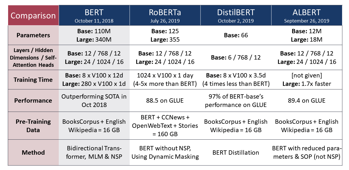
3.7 Comparing RoBERTa, DistilBERT and ALBERT
Summarizing the theory, each of the three presented BERT-based models has their own modifications and promises very good performances - which we will test in the next chapter. For easy comparison, we summarized the model differences in the table below (adapted and extended from Khan’s (2019) summary here.
4. Application to Economic Policy Uncertainty
After understanding the transformer-based models in theoretical context, we apply them to our classification problem: to determine if there is economic uncertainty in newspaper articles with the aim of extending and improving the current classification methodologies. For this purpose, we use the package Simple Transformers, which was built upon the Transformers package (made by HuggingFace). Simple Transformers supports binary classification, multiclass classification and multilabel classification and it’s wrapping the complex architecture of all of the previously mentioned models (and even more!). SimpleTransformers requires only three essential lines of code to initialize, train and evaluate the model and obtain ready-to-go transformers. Using this package, transformer models can relatively easily be applied in research and business contexts - which we will subsequently demonstrate. For implementation, we recommend the authors’ blogpost as a starting point.
4.1. Data Preparation
4.1.1 Data Exploration
The original dataset we used was labeled and consisted of three columns:
(i) Article ID
(ii) Article - the newspaper articles in text format
(iii) label - a binary indicator showing if the article is related to economic policy uncertainty or not.
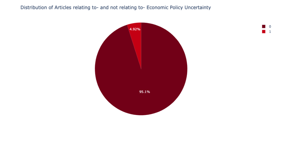
The entire dataset contains 50,483 articles and is imbalanced, with only about 5% of the articles being marked (1), related to economic policy uncertainty.
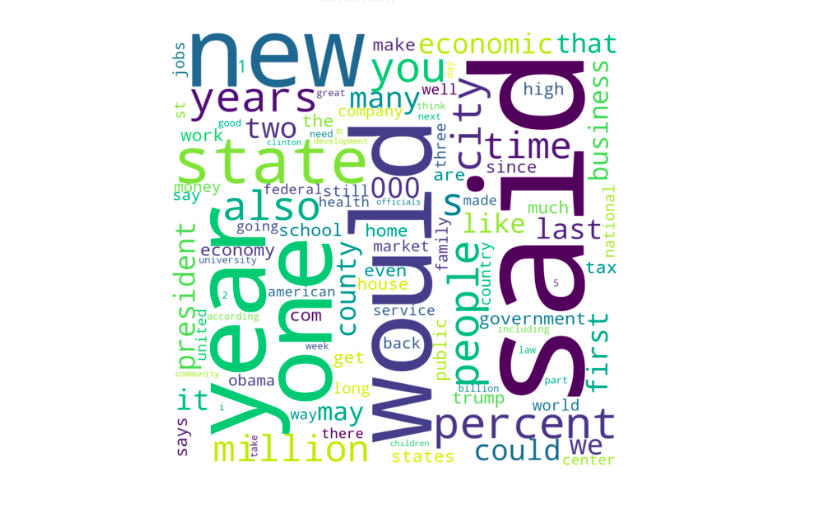
All articles are written completely in English. The average length of the newspaper articles is 534 words (after cleaning).
Overall, after removing punctuations, stop words and fixing the (i’d, she’d, etc), the following top words appear:
4.1.2 Data Pre-Processing
We applied the standard text cleaning procedures to the articles. All text was made lower case, punctuation removed, HTML links/email addresses removed. We also removed numbers.
Since the data originated from a replication of Baker et al.‘s methodology, the labeling of the data are assumed to come from the presence of either of the three words “economic” , “policy”, or “uncertainty”. Thus, we removed these words from the train set while considering the modeling part. In such scenarios, we believed that the presence of these three tokens while training would cause overfitting.
We restricted the number of words for an article to 200 while modeling, which we discuss further in the modeling section.
4.1.3 Data Imbalance
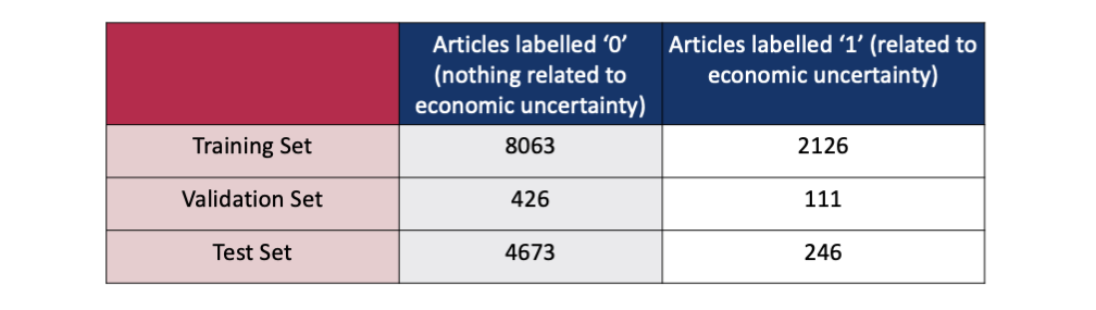
The data imbalance in the original dataset was 95% labeled as “0” and 5% as “1”. However, instead of generating synthetic samples to regenerate the data, we opted to rebalance the dataset. We balanced the training and validation set on almost 80-20 ratio of 0:1. This was to ensure that the models will have enough samples to learn. However, for the test set we maintained the original imbalance ratio which was 95:5. The following table illustrates the rebalancing.
4.2. Models Implementation
For the binary task of economic policy uncertainty determination, we use the previously introduced BERT-based models:
- BERT
- DistilBERT
- RoBERTa
- ALBERT
We compare their performance to two baseline models: a bidirectional neural network and a SVM classifier.
4.2.1 Transformer-based Models
The Simple Transformers package lets us train, evaluate and test our models. We show our implementation on the example of RoBERTa. All the steps presented in the notebook below were also applied to BERT, DistilBERT and ALBERT with the same hyper-parameters, differing only in the line of code that specifies the model. For example, the Classification Model function can take in “bert” instead of “roberta” and “bert-base-uncased” instead of “roberta-base” to run the BERT model.
Parameters in Simple Transformers:
BERT-based models come with a set of hyper-parameters which need to be adjusted properly for the task. With the Simple Transformers package, one is able to set these directly by passing values, as mentioned in the authors’ blog post. The full list of the setting with detailed description can be found on the author’s website. For our binary classification approach, we replaced the hyper-parameters’ default values for the most impactful ones:
- Number of training epochs: The epochs were increased from 1 to a number as high as 10. However, increasing the number of epochs also increased the running time of the model intensively. At the end, 4 epochs turned out to be the most optimal number, balancing between running time and giving good results.
- Batch size: The batch size was increased from 2 till 16, and batch size of 8 gave good results. With a batch size of 4, we observed a certain overfitting.
- Maximum Sequence Level: Although the model can handle a maximum of 512 tokens, we started off first with 100 tokens, and then opted for 200 tokens. The average length of the articles in the entire dataset was 534, which implies that setting this hyper-parameter to 512 could have been an ideal choice. However, owing to certain computational difficulties it was limited to 200.
- Learning Rate: 4e-5. Changing this learning rate made the model run either faster or slower, results were optimal for this chosen learning rate.
4.2.2 Benchmarks
Transformer based models often come with high training times and the results can be a matter of speculation, depending on the training dataset and if a transfer learning approach has been used. Therefore, we compare the performance to two non-transformer based models as well. We have used a small bidirectional neural network and a SVM classifier.
4.2.3 Interpretation of Results
In datasets having a high imbalance like the one we used, accuracy is not the right metric to assess model performance with. For example, if all articles are classified as “0” (not being related to economic policy uncertainty), then the accuracy is 95%. This seems like a very favorable result, when in reality no single article is classified as “1” and the model is actually very bad. Therefore, we decided to use the following other metrics for this purpose:
-
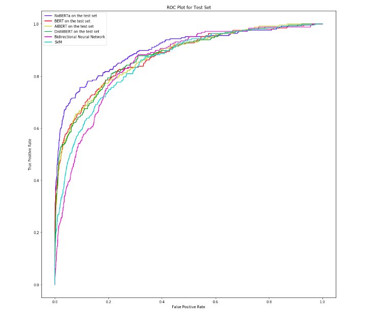
Area Under Curve (AUC) is a measure that takes into account the true and false positives. It measures the area under the (ROC) curve, which plots the false positive rate (specificity) against the true positive rate (sensitivity). A perfect model would have an AUC of 1, a randomly assigning model would be at 0.5.
-
F1-Score (F1) balances between precision (= True positives /(True positives + False positives) ) and recall (= True positives /(True positives + False negatives) ) and ranges from 0 to 1 - the higher the better.
-
Matthew’s Correlation Coefficient (MCC) uses all four measures - true positives, true negatives, false positives and false negatives - in its calculation. The score goes from -1 (everything is wrongly classified) to 1 (everything is correctly classified).
The following result table was calculated based on the standard binary cut-off of 0.5. If the probability (converted from the log-odds output of the model) is greater than 0.5, the article is labeled as related to economic policy uncertainty and marked as “1”, otherwise it is marked as “0”. This cutoff of 0.5 was maintained across all models to provide a standard comparison. We will address whether this cut-off is optimal or not in the discussion section.
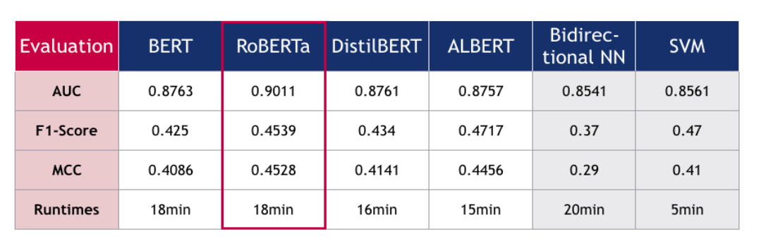
From the table we can see that the BERT-family models all perform better than the benchmark models. While BERT’s, DistilBERT’s and ALBERT’s performance does not differ much from each other across all of our metrics (AUC of around 0.87), RoBERTa largely outperforms them. Their runtimes were similar around 18 minutes, with DistilBERT and ALBERT being slightly faster, and the SVM taking by far the least time with only 5 minutes runtime.
The benchmarks performed very close to the other BERT family models, apart from RoBERTa. This is indeed very interesting to observe that relatively less “complex” models have comparable AUC, F1-score and MCC. This might have to do with the parameters of the benchmarks:
- The first benchmark was a bidirectional neural network with LSTM, where the maximum length was kept to 200, in line with BERT models. The number of layers and maximum length can also be tuned in a way, to perform almost the same as BERT, but this causes overfitting on the test set.
- The other benchmark was SVM, whose tuning was kept to the minimum. The intention was to observe how the results would be like on default functions, without tuning.
Although the above results are taken for certain hyper-parameters kept constant across all BERT-family models (for example the epoch, training batch size, maximum sequence length), we observed that changing these parameters causes a change in the results. For example, running the models for higher epochs caused heavy overfitting with the difference between the F1-score between training set and test set being more than ~0.5. In view of these considerations, it could be concluded that results are partly dependent on hyper-parameter tuning.
Overall, these observed results theoretically make sense: RoBERTa is the largest model, trained on the largest datasets and can therefore perform very well. DistilBERT and ALBERT both balanced a high performance with size and speed of the model - and their performance is indeed a little lower, while they took less time to run. On the whole, all models perform remarkably well - a promising result for future researchers of economic policy uncertainty!
5. Further Discussion
Several choices and observations in our application call for further discussion, because they can still be optimized depending on the application at hand or need to be taken with caution.
5.1 Optimal Threshold Calculation
The simple transformers library uses a cut off of 0.5 as decision criteria while calculating the results. Probability greater than or equal to 0.5 is labeled as “1”, else labeled as “0”. However, the best cutoff heavily depends on the use case (for example, if one wants to identify the 1’s more than the 0’s would focus on precision). In certain business scenarios, there might be high costs for false negatives or false positives. In our case, rather than high costs with just false positives or false negatives, we think it is necessary to identify both types of articles correctly. Yet the cut-off of 0.5 might not exactly be optimal for highly imbalanced datasets. In order to see how the other metrics would vary with changing the cut-off, we chose the best performing model from above and observed how the metrics varied.
Although the simple transformer library gives result tables for 0.5, for deciding the optimal cutoff we have taken the log-odds output from the model and then converted it into probabilities.
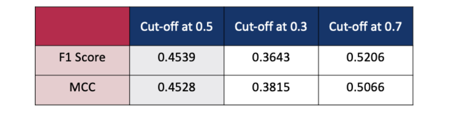
As the cutoff is increased from 0.5 to 0.7, there is some improvement in the F1 Score and MCC. However, if the cutoff is increased to 0.8, both of the metrics show a decline. Similarly, lowering the cut-off from 0.5 to 0.3 also results in a considerably low F1 Score and MCC. If the task involves capturing most of the true positives (articles related to economic policy uncertainty) then a cut off of 0.3 identifies more articles (192 True Positives) than the 0.5 cutoff (182 True Positives). Choosing a right-cutoff will involve trade-off between accuracy, F1-Score and MCC and would highly depend on the task at hand.
5.2 Impact of Certain Tokens in Identifying Uncertainty
Another step that can largely influence the model results is done at the very beginning: preprocessing of the data. Although these steps involve removing stop words, punctuation and giving ~200 words as input to the models, there is a high chance that certain words might be heavily influencing the identification of economic policy uncertainty related articles. In order to investigate this, we first observed the top occurring words in the training set. Based on the observations, we grouped certain words/tokens into “general” and “data specific”.
- general words/tokens- “would” , “said”, “year” , “new”, “one”
- data specific words/tokens- “usa”, “trump”, “president”.
These word/tokens groups are called “general” and “data specific” due to their nature of language. General words/terms would occur in any type of text not related to economic policy uncertainty. However, the “data specific” terms would occur often in text related to global economic topics. Our aim was to check how the presence and absence of these words/tokens would impact the result metrics. For this purpose we chose RoBERTa, our relatively best performing model and kept all hyper-parameters constant for tuning, and also a cut off of 0.5 for the decision threshold.
-
In the first case, we drop the “general” tokens from the training set, which were “would” , “said”, “year” , “new”, “one” and train RoBERTa, but retained the “data specific” tokens.
-
In the second case, we drop the “data specific” which were “usa”, “trump”, “president”, tokens from the training set, however retaining the “general” tokens.
-
The following changes are observed on the test set, in which the “general” or “data specific” tokens are not dropped in any case.
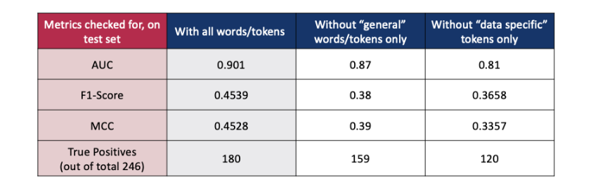
When certain word/token groups are removed from the training set, we see that there is a drop in all metrics on the test set. The drop is even more significant when the “data specific” words/tokens are removed. This also partially confirms the original idea, that including “economic”, “policy”, and “uncertainty” keywords would have overfitted the model and give a lot of false positives, after all these words/tokens are also part of “data specific” tokens.
At this point, it should be noted that the entire newspaper articles are “loosely” related to economic policy and uncertainty (including ones labeled as “1” and “0”), so there would be certain data biases in words and tokens recurring frequently. This word/token group approach opens our minds to infinite possibilities, such as which words or which word groups are really contributing to the overfitting of the model, and lead to other areas of investigation. However, we conclude that presence and absence of certain word/tokens or combinations do have an impact on how good the classifier is.
Lastly, it is important to take into account that in a transfer learning approach, results also depend on the data the original model has been trained on. Since RoBERTa has been trained on a huge English language corpus and our data is in English, it works well. But, if we had a German data set, would these models have given a good result?
6. Conclusions
In this project, we aimed to identify economic policy uncertainty in newspaper articles using state of the art NLP models. Starting off with Baker et al.‘s (2016) simple and manual method to classify articles, we illustrated how NLP models can compete with other, potentially costly data labeling methods and thereby open up new research possibilities. In order to do so, we explored how BERT and three BERT-based transformer models approach text classification. RoBERTa, DistilBERT, and ALBERT each improve the original model in a different way with regards to performance and speed. In our application, we demonstrated the easiest way to implement transformer models, how to modify the standard settings and what else to pay attention to. On the task of identifying economic uncertainty, RoBERTa - the biggest model with the largest training data - performed best. However, the field of NLP is fast moving - and we are excited to see what the next transformational generation of models will bring.
7. References
Alammar, Jay. 2018a. “The Illustrated Transformer.” June 27, 2018. http://jalammar.github.io/illustrated-transformer/.
—. 2018b. “The Illustrated BERT, ELMo, and Co. (How NLP Cracked Transfer Learning).” December 3, 2018. http://jalammar.github.io/illustrated-bert/.
—. 2019. “A Visual Guide to Using BERT for the First Time.” November 26, 2019. http://jalammar.github.io/a-visual-guide-to-using-bert-for-the-first-time/.
B, Abinesh. 2019. “Knowledge Distillation in Deep Learning.” Medium. August 30, 2019. https://medium.com/analytics-vidhya/knowledge-distillation-dark-knowledge-of-neural-network-9c1dfb418e6a.
Baker, Scott, Nicholas Bloom, and Steven Davis. 2016. “Measuring Economic Policy Uncertainty.” The Quarterly Journal of Economics 131 (4): 1593-1636.
Devlin, Jacob, Ming-Wei Chang, Kenton Lee, and Kristina Toutanova. 2019. “BERT: Pre-Training of Deep Bidirectional Transformers for Language Understanding.” ArXiv:1810.04805 [Cs], May. http://arxiv.org/abs/1810.04805.
Huang, Cary. 2019. “How the Winds of Political Uncertainty Are Battering the Global Economy.” South China Morning Post, October 30, 2019. https://www.scmp.com/comment/opinion/article/3035226/us-china-trade-war-trumps-impeachment-inquiry-and-brexit-record.
Khan, Suleiman. 2019. “BERT, RoBERTa, DistilBERT, XLNet - Which One to Use?” Medium. September 4, 2019. https://towardsdatascience.com/bert-roberta-distilbert-xlnet-which-one-to-use-3d5ab82ba5f8.
“Knowledge Distillation - Neural Network Distiller.” n.d. Nervanasystems on Github. Accessed December 3, 2019. https://nervanasystems.github.io/distiller/knowledge_distillation.html.
Lan, Zhenzhong, Mingda Chen, Sebastian Goodman, Kevin Gimpel, Piyush Sharma, and Radu Soricut. 2019. “ALBERT: A Lite BERT for Self-Supervised Learning of Language Representations.” ArXiv:1909.11942 [Cs], October. http://arxiv.org/abs/1909.11942.
Liu, Yinhan, Myle Ott, Naman Goyal, Jingfei Du, Mandar Joshi, Danqi Chen, Omer Levy, Mike Lewis, Luke Zettlemoyer, and Veselin Stoyanov. 2019.
“RoBERTa: A Robustly Optimized BERT Pretraining Approach.” ArXiv:1907.11692 [Cs], July. http://arxiv.org/abs/1907.11692.
“Pretrained Models - Transformers 2.2.0 Documentation.” n.d. Accessed December 3, 2019. https://huggingface.co/transformers/pretrained_models.html.
Sanh, Victor. 2019a. “The Best and Most Current of Modern Natural Language Processing.” Medium (blog). May 22, 2019. https://medium.com/huggingface/the-best-and-most-current-of-modern-natural-language-processing-5055f409a1d1.
—. 2019b. “Smaller, Faster, Cheaper, Lighter: Introducing DilstilBERT, a Distilled Version of BERT.” Medium (blog). August 28, 2019. https://medium.com/huggingface/distilbert-8cf3380435b5.
Sanh, Victor, Lysandre Debut, Julien Chaumond, and Thomas Wolf. 2019. “DistilBERT, a Distilled Version of BERT: Smaller, Faster, Cheaper and Lighter.” ArXiv:1910.01108 [Cs], October. http://arxiv.org/abs/1910.01108.
Tobback, Ellen, Hans Naudts, Walter Daelemans, Enric Junque de Fortuny, and David Martens. 2018. “Belgian Economic Policy Uncertainty Index: Improvement through Text Mining.” International Journal of Forecasting 34 (2): 355-65. https://doi.org/10.1016/j.ijforecast.2016.08.006.
Vaswani, Ashish, Noam Shazeer, Niki Parmar, Jakob Uszkoreit, Llion Jones, Aidan N. Gomez, Lukasz Kaiser, and Illia Polosukhin. 2017. “Attention Is All You Need.” ArXiv:1706.03762 [Cs], December. http://arxiv.org/abs/1706.03762.
“What Is Brexit-Related Uncertainty Doing to United Kingdom Growth?” 2016. Economic Policy Uncertainty. May 16, 2016. http://www.policyuncertainty.com/brexit.html.