By Seminar Information Systems (WS 19/20) | February 7, 2020
Table of Contents
- Generating Synthetic Comments to Balance Data for Text Classification
- Byte Pair Encoding
- Comparing Generated Text
- Comment Classification Task
- Relation to Business Case
- Classification Approach
- Classification Architecture
- Classification Settings
- Drawbacks of Oversampling with Generated Text
- Classification Task - Limitations
- Evaluation
- Including the “Not-Sure”-Category
- Different Balancing Ratios for Generated Comments
- Conclusion and Discussion of Results
- References
Generating Synthetic Comments to Balance Data for Text Classification
Lukas Faulbrück
Asmir Muminovic
Tim Peschenz
Introduction
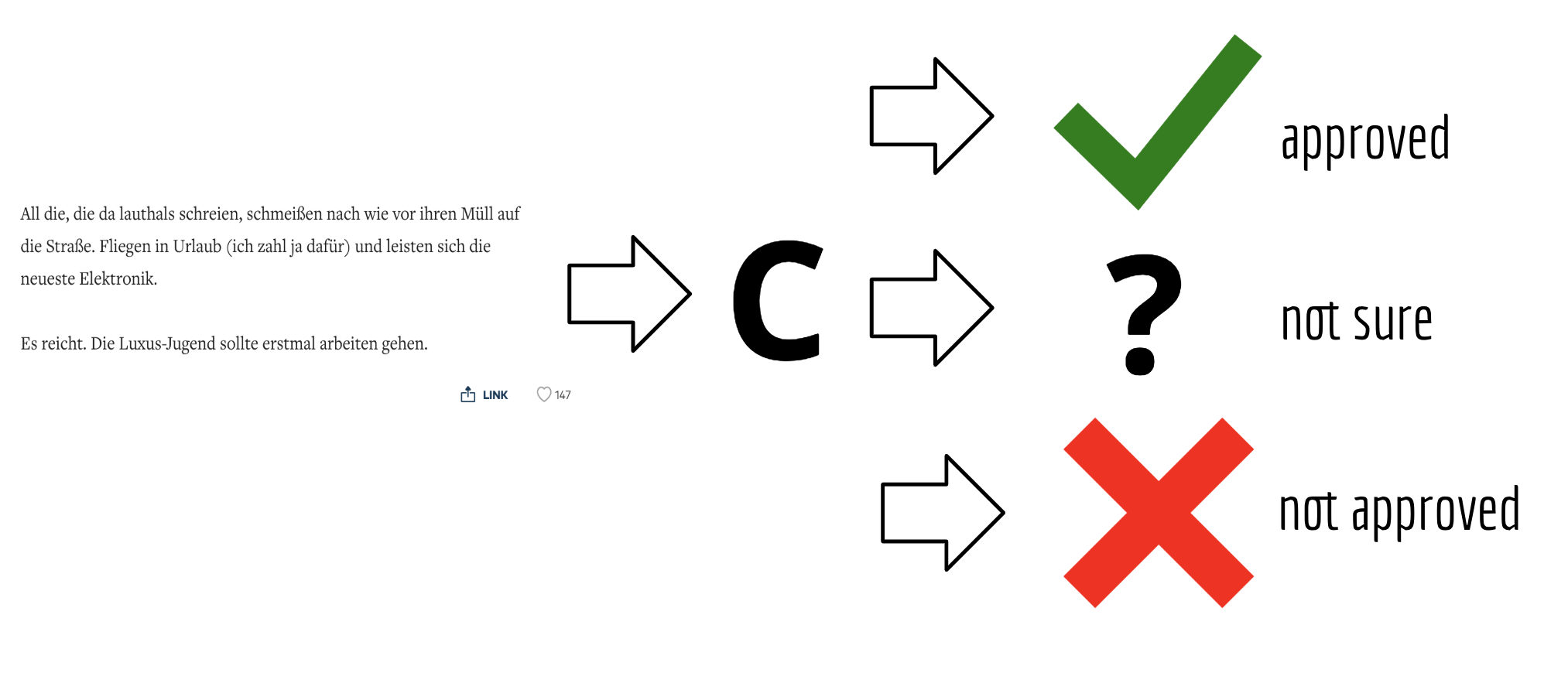
In the age of social networks, a strong and active community is an important part for a company to spread its brand. Many companies have therefore established a commentary function which serves as a discussion platform. Especially newspaper publishers use the commentary function for their online articles. A big problem that these companies have to face are comments that are not compatible with their guidelines. It includes racist, insulting or hate-spreading comments. Filtering all these comments by hand requires enormous human resources. One person can review an average of 200 to 250 comments per day. With 22,000 comments per day, which is a realistic number, a company needs to pay about 100 employees daily. To reduce this number and the associated costs, there is the possibility to build a classifier which predicts whether a comment is approved, whether it should be blocked or whether a human should check it again. There are already some scientific papers that have dealt with this very subject (Georgakopoulos et al., 2018; Ibrahim et al., 2018; van Aken et al., 2018). With the help of this existing work, companies can build a classifier that is adapted to their needs.
At an average cost of 16€/h per employee and an 8 hour working day, a company must pay a total of 12,800€ per day for 100 employees. If it is possible to reduce the comments to be reviewed to 20%, the company can save a total of 10,240€ in costs per day. This saves on personnel costs, company compliance goals are achieved and the user is also satisfied because her/his comment can be posted directly online.
In the course of the blog a classifier will be built, which should solve the described problem. Only the text is used as input for the model in order to investigate the effects of the text isolated from other features. However, it should be mentioned that other features such as the length of the text, the number of comments posted by a user or the frequency of punctuation marks can also have a positive influence on a classifier.
Data Exploration
In the further work a data set is used, which contains among other attributes the comments, which were posted in the comment section of a German newspaper. In total, the data set contains four attributes. The first attribute shows the date on which the comment was posted. This is used to filter a period from May 2018 to April 2019. The second attribute is a binary indicator about the customer status (subscriber/not subscriber). In order to limit the focus on one target group, only the subscribers are used for further tasks. The third attribute is the main feature and contains the actual text (comment). The last attribute is the label, which we need for the classifier. It indicates whether a comment is publishable or not.
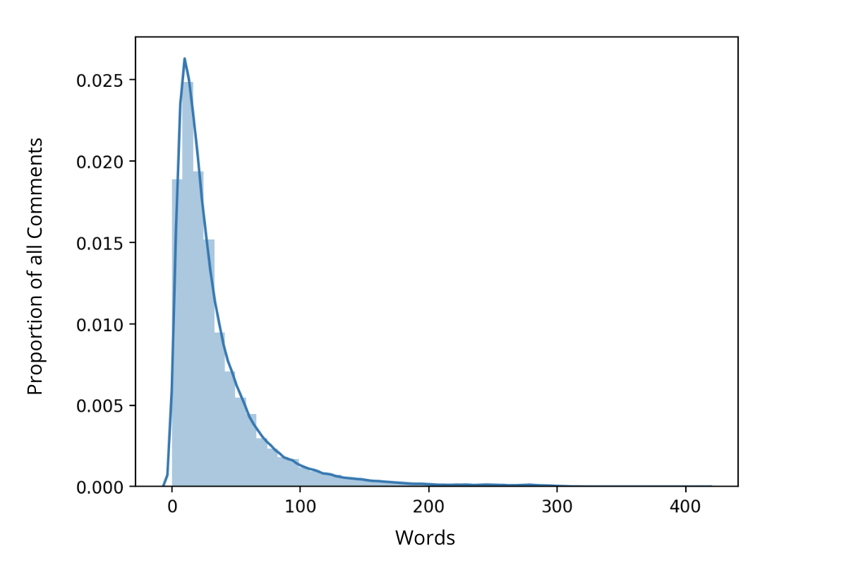
The next figure shows the distribution of the length of the not publishable comments. You can see that most of the comments have a length between 10 and 100.
A closer look at the distribution of the publishable and not publishable comments shows that there is an imbalance between these two classes.
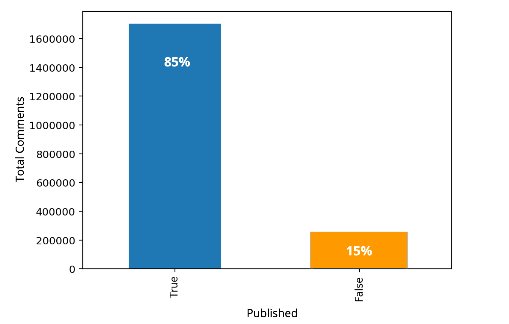
In total, we have 1,62 million comments labeled as published and about 280,000 comments labeled as not published. Classification of data with imbalanced class distribution has encountered a significant drawback of the performance attainable by most standard classifier learning algorithms which assume a relatively balanced class distribution and equal misclassification costs (Yanmin Sun et al., 2007). There are different ways to deal with unbalanced data. Basic methods for reducing class imbalance in the training sample can be sorted in 2 groups (Ricardo Barandela et al., 2004):
- Over-sampling
- Under-sampling
Undersampling is a popular method in dealing with class-imbalance problems, which uses only a subset of the majority class and thus is very efficient. The main deficiency is that many majority class examples are ignored (Liu et al., 2009). Oversampling on the other hand replicates examples in the minority class. One issue with random naive over-sampling is that it just duplicates already existing data. Therefore, while classification algorithms are exposed to a greater amount of observations from the minority class, they won’t learn more about how to tell original and non-original observations apart. The new data does not contain more information about the characteristics of original transactions than the old data (Liu et al., 2007).
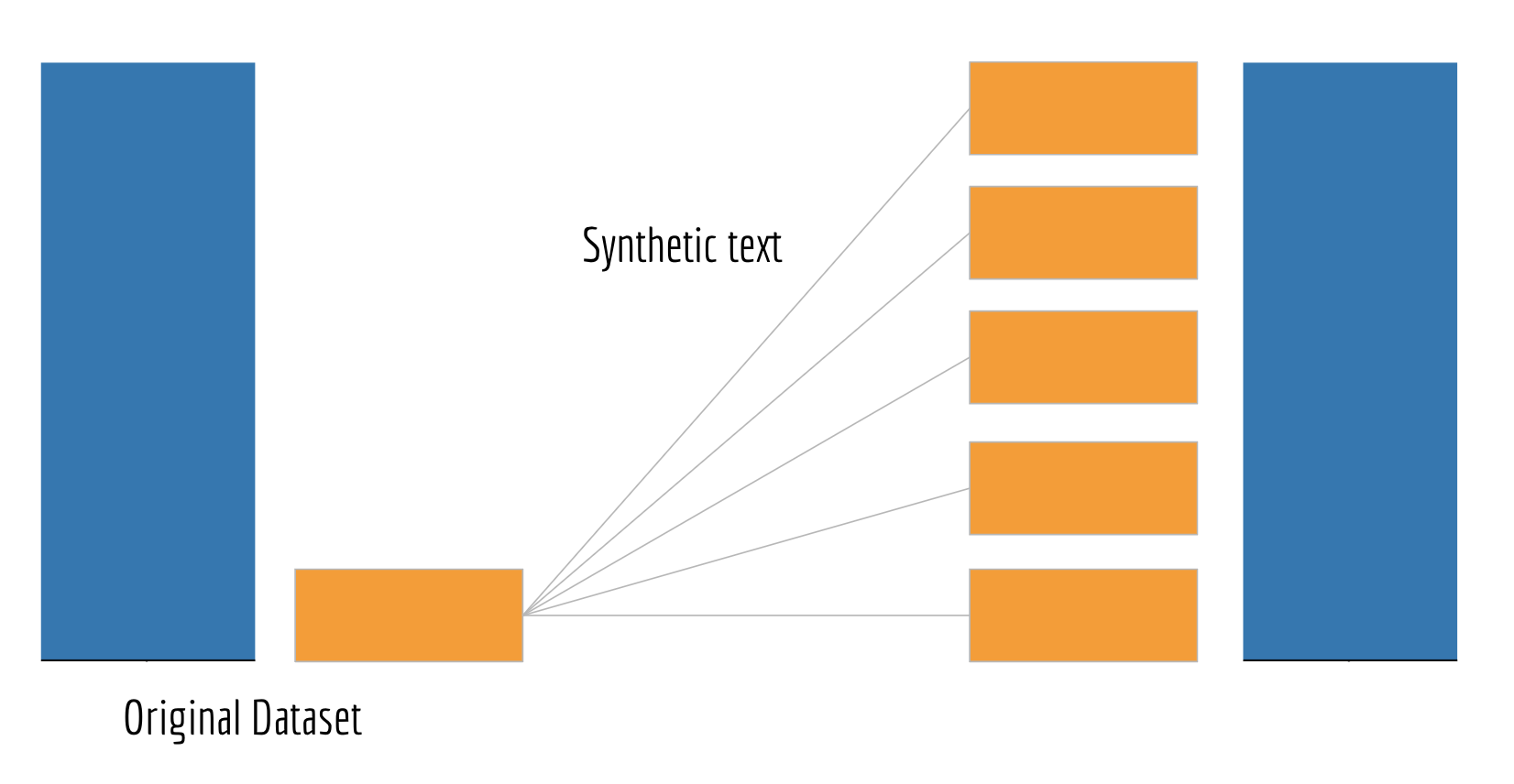
To balance our data set, we have decided to use a form of over-sampling. We generate synthetic text using language models that take the minority class as input and add the generated comments to original observations. By this method we don’t have duplicates of the observations from the minority class, but new comments that take the same properties of the minority class (Stamatatos, 2007). By creating sythetic text instead of just reusing it, our classifier is less likely to overfit. At the same time we need to make sure that the generated comments are realistic. In our case realistic means that it could been written by a human being.
It is not necessarily the best way to balance the data set so that the final ratio is 50:50. The trade-off between introducing noise through text generation and the benefits of oversampling the minority class needs to be accounted for. Therefore, it could be beneficial to only balance out the classes to a certain degree, in that way we would avoid introducing too much noise but still yield the benefits of oversampling.
When generating the text we decided to compare two language models with each other. One is a keras language model, used in generation and training. It is sequence to sequence model using a bilayer encoder and decoder with dropout and a hidden dimension of 128. The second language model we are using is GPT-2. The Generative Pre-Training version 2 was developed by OpenAI and is a state-of-the-art language model that can generate text. A detailed explanation of GPT-2 will be given in a later part of the blog.
Data Pre-Processing
Before the generation of comments can begin, the data must first be prepared. We will not explain all pre-processing steps, but focus on the central ones.
First we split our data into a train and test set.
The test set won’t be touched until the very end when we are doing the evaluation.
A key to generating good comments is the preparation of the text. For this purpose we have defined two functions. One function prepares the text for the generation part and the other function for the classification.
The different steps in the preparation of the text can be discussed. Especially the removal of punctuation marks can lead to worse results when generating new comments. For the blog post, we stick to the steps shown. But for future research it can be experimented with different text pre-processing steps.
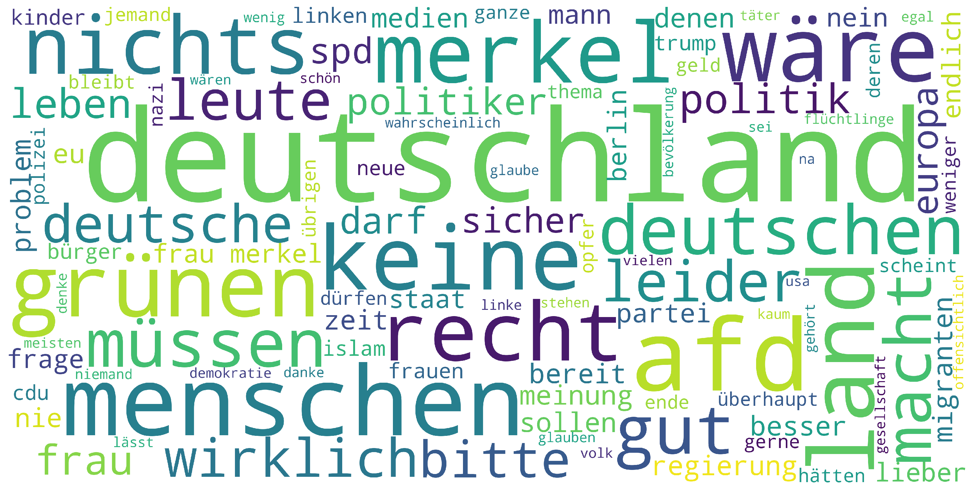
The following word cloud shows the most used words in the class of not publishable comments after cleaning and removing some common words (to get a clearer word cloud).
While exploring and pre-processing the text, we have noticed some points that can have a negative impact on the performance of our models. Not all comments that are labeled as not publishable can be guaranteed to be so. We have read some comments where, without knowing the context, it was difficult to understand why they were labelled as not publishable. For example, the comment ‘Und wer ist der Papa?’ (‘And who is the daddy?') may not look not publishable at first glance, but may be inappropriate in the context. Another critical point is the vocabulary of the users. Some words are used which only occur in the cosmos of the comment section. This can become a problem if a pre-trained embedding is used which was trained in another context. The last point, which can have a negative impact, are many spelling mistakes made by the users. Pre-trained embeddings will probably not recognize words with spelling mistakes and self-trained embeddings will represent these words as individual vectors. For now we ignore that potential problems but have to keep that in mind for evaluation as well as for future steps.
Text Generation
For the text generation we compare two language models. A Language Model is taking a text sequence as an input and predicts the next word for that sequence. A popular example of a Language Model is the next word suggestions feature in Today´s smartphones.
In order to better understand where we are in the world of embeddings, we have marked the two important places in the following graphic in red. The graphic was created by Andrien Sieg which blog post you can find here link.
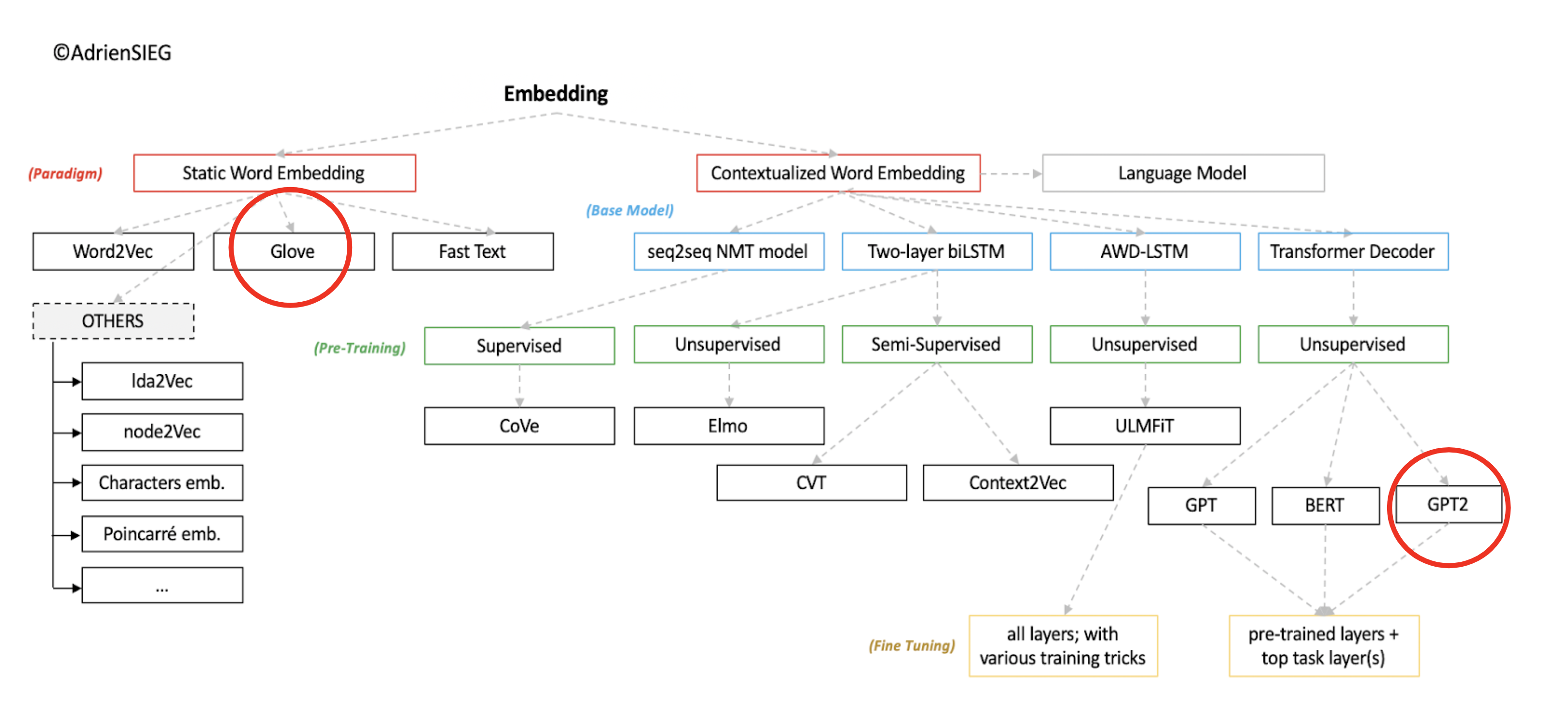
Image Source 1)
Language Model - GloVe
The first model is a sequence to sequence model. It takes a sequence as an input and generates a new sequence (the words of our new comment). A sequence to sequence model has two components, an encoder and a decoder. The encoder encodes the input sequence to a vector called the context vector. The decoder takes in that context vector as an input and computes the new sequence. A disadvantage of this structure is that the context vector must pass all information about the input sequence to the decoder. So that the decoder is not only dependent on the context vector, but gets acess to all the past states of the encoder, we implement an additional Attention Layer, which takes over this task. The function and idea of the Attention Layer, which we use here, was introduced by Luong et al. (2015). How Attention works in detail is explained in a later part of the post when GPT-2 takes it’s turn.
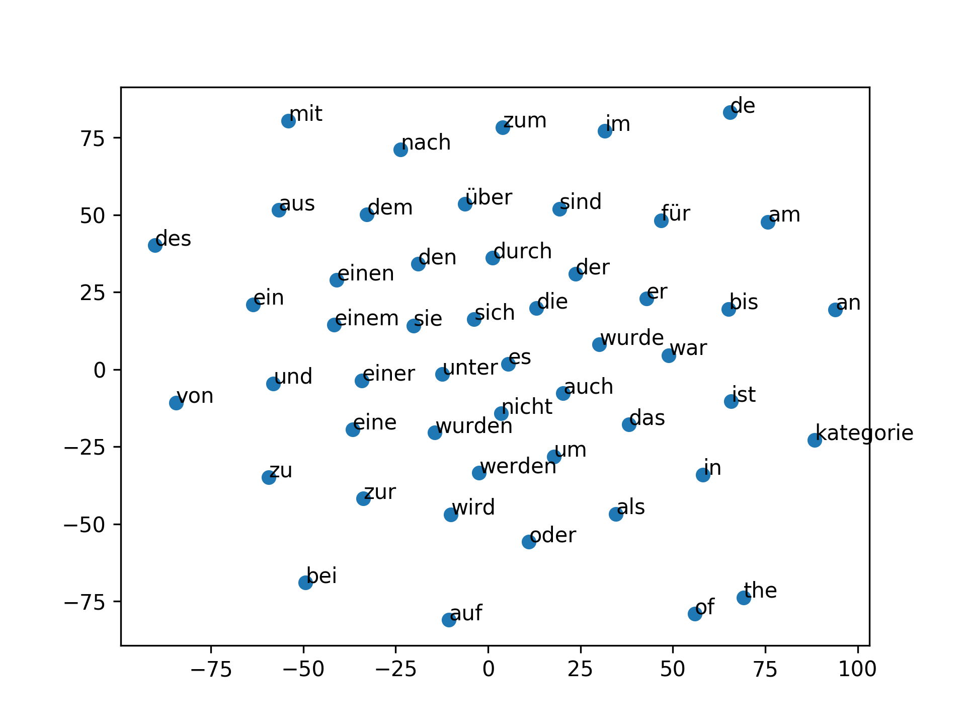
In order to represent our words we use a pre-trained German GloVe embedding from deepset link. It was trained on a German wikipedia corpus in 2018. The following graphic visualizes the connections of the words in space. The visualization is limited to 50 words.
We will not give a detailed description of embeddings in our blog, as this topic is a blog post in itself, but a very good explanation is given by Allen and Hospedales (2019), which can be found in the references.
Further Text Preparation
For our first model some additional steps have to be taken to prepare the input for the model. We set a training length at 15. The training length is a parameter that plays an important role in the generation of the text. With a higher training length we give our model more information to predict a word. However, we also lose some observations that do not meet the minimum length to use them for the defined training length. Furthermore, we turn our texts into sequences of integers. These steps and some more are shown and briefly explained in the following function.
Next we need to create the features and labels for both the training and validation. Since our model will be trained using categorical cross entropy we need to convert the labels in one hot encoded vectors.
The next step is loading the German GloVe embedding and creating an embedding matrix. In addition, we check how many words without pre-trained embeddings exist. In total, about 40% of the words in the comments are not covered by the embedding. That are a lot of words, which leads to a loss of information. The reason for this are the problems already mentioned at the end of the exploring part. The context in which the embedding was trained (wikipedia) is different from the vocabulary of the users in our comment section. Furthermore, words with spelling mistakes do not exist in the embedding and are counted as separate words, even if the correctly spelled word occurs in the embedding. A solution to this problem is to train an own embedding based on the comments, which can be expensive. However, for the generation of the text we continue with the pre-trained embedding.
Modeling
After we have completed all the necessary steps, we can start building the architecture of our recurrent neural network.
After converting the words into embeddings we pass them to our encoder and decoder block. The encoder consists of a bidirectional LSTM layer and another LSTM layer with 128 nodes each. LSTM (Long Short Term Memory) is a type of recurrent neural network introduced by Hochreiter & Schmidhuber (1997). As an RNN it has a word as an input instead of the entire sample as in the case of a standard neural network. This ability makes it flexible to work with different lengths of sentences. The advantage of LSTM against RNN is the ability to capture long range dependencies. Since we are interested in the whole context of a comment that memory is very useful. Bi-Directional brings the ability to work with all available information from the past and the future of a specific time frame (Schuster and Paliwal, 1997). The decoder consists of two LSTM layers also with 128 nodes. Both the encoder and the decoder use dropout to prevent overfitting. Return_sequences is set to true so that the next layer has a three-dimensional sequence as input. Next we give the attention layer as input the output from the encoder and decoder. The output of the attention layer must then be merged with the output of the decoder. Before we can feed the output to our final layer we have to make sure that it has the right shape. Our last layer is the prediction layer using softmax as an activation function.
For the loss function we have chosen categorical crossentropy. It is used in classification problems where only one result can be correct.
Where:
M - number of classes
N - number of samples
ŷ - predicted value
y - true label
log - natural log
i - class
j - sample
Categorical crossentropy compares the distribution of the predictions (the activations in the output layer, one for each class) with the true distribution, where the probability of the true class is set to 1 (our next word) and 0 for the other classes (all the other words). The closer the model’s outputs are to the true class, the lower the loss.
As an optimizer we use Adam optimizer (Adaptive Moment Estimation) which computes adaptive learning rates for each parameter. That algorithm is used for first-order gradient-based optimization of stochastic objective functions (Diederik P. Kingma and Jimmy Ba, 2014). As an evaluation metric we use accuracy.
Now that we have built our model we can train it for a fixed number of epochs. We use callbacks to save the best model and to stop the training if there is no improvement of the validation loss after 5 epochs. After we have trained our model we evaluate it.
With our first model we achieve a cross entropy of 7.2, which can be interpreted as average performance. Very good text generation is achieved with a cross entropy of about 1.0.
Generation
After we have finished training our neural network, we can start generating text. To do this, we first choose a random sequence, from the sequences we have defined in one of the previous steps. From this sequence we use 15 contiguous words as seed. This seed is then used as input for the model to predict the 16th word. The 16th word is appended to the last 14 words of the seed, so that we again have 15 words as input for the model to predict the 17th word. This procedure is continued until a length is reached that matches the length of a randomly selected not publishable comment. For the choice of the generated word, we have also implemented temperature. It defines how conservative or creative the models’s guesses are for the next word. Lower values of temperature generates safe guesses but also entail the risk that the same words occur frequently or that these words are repeated. Above 1.0, more risky assumptions are generated, including words that increase the diversity of the generated comment.
With the help of the defined function, new comments are created and saved as csv in order to use them later for classification.
One question that needs to be asked after text generation is what metric is used to evaluate the quality of the text. One of the most popular metrics for evaluating sequence to sequence tasks is Bleu (Papineni et. al, 2002). The basic idea of Bleu is to evaluate a generated text to a reference text. A perfect match results in a score of 1.0, whereas a perfect mismatch results in a score of 0.0. However, it has some major drawbacks especially for our use case. A bad score in our case does not necessarily mean that the quality of our generated comment is poor. A good comment looks as if it was written by a human being. To check the quality of the comments, we decided to read some of them randomly. In order to check the quality of the comments, we decided to read some of them randomly to see if the comments sound realistic. Two samples for a good and a bad one are shown after the GPT-2 part.
Language Model GPT-2
GPT-2 is an unsupervised Transformer language model, more specifically a Generative Pre-trained Transformer. The second of its kind, thus the name GPT-2. This model was first introduced in a paper called ‘Language Models are Unsupervised Multitask Learners’ by A. Radford et al. (2019).
Why GPT-2?
GPT-2 is capable of delivering state-of-the-art performance across many different tasks, such as text generation, question-answering, reading comprehension, translation and summarization – all without task-specific training (Radford et al., 2019). We wanted to leverage the text generation qualities of GPT-2 to our advantage.
What makes GPT-2 so powerful?
What makes GPT-2 so powerful is its sheer size. It was one of the biggest models at the time of the release, the full model has 1.5 Billion parameters, which makes it about five times bigger than its previous iteration GPT (Radford et al., 2018). It was trained on an as large and diverse dataset as possible with the objective to collect natural language demonstrations of tasks in varied domains and contexts (Radford et al., 2019). The dataset is known as WebText and has 40 GB of text data.
The Problem of Long-Term Dependencies
Since a language model is trying to predict the next word based on previous words, context becomes very important. Let´s imagine this toy example “the lead singer of the…”, it is obvious that the next word has to be “band”.
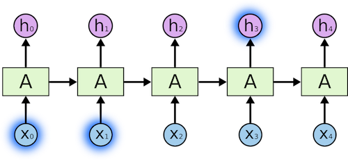
Image Source 2)
In this case, the relevant information and the word to predict are close, RNNs (or CNN) can learn to use past information and find out what is likely to be the next word for this sequence. Now, with a longer sentence. Let´s say we are predicting the next word in “I grew up in Spain… I speak fluent…”.
The recent words indicate that the word to predict next should be a language, but to know what language specifically, there is a need for context of Spain, that is further back in the sequence.
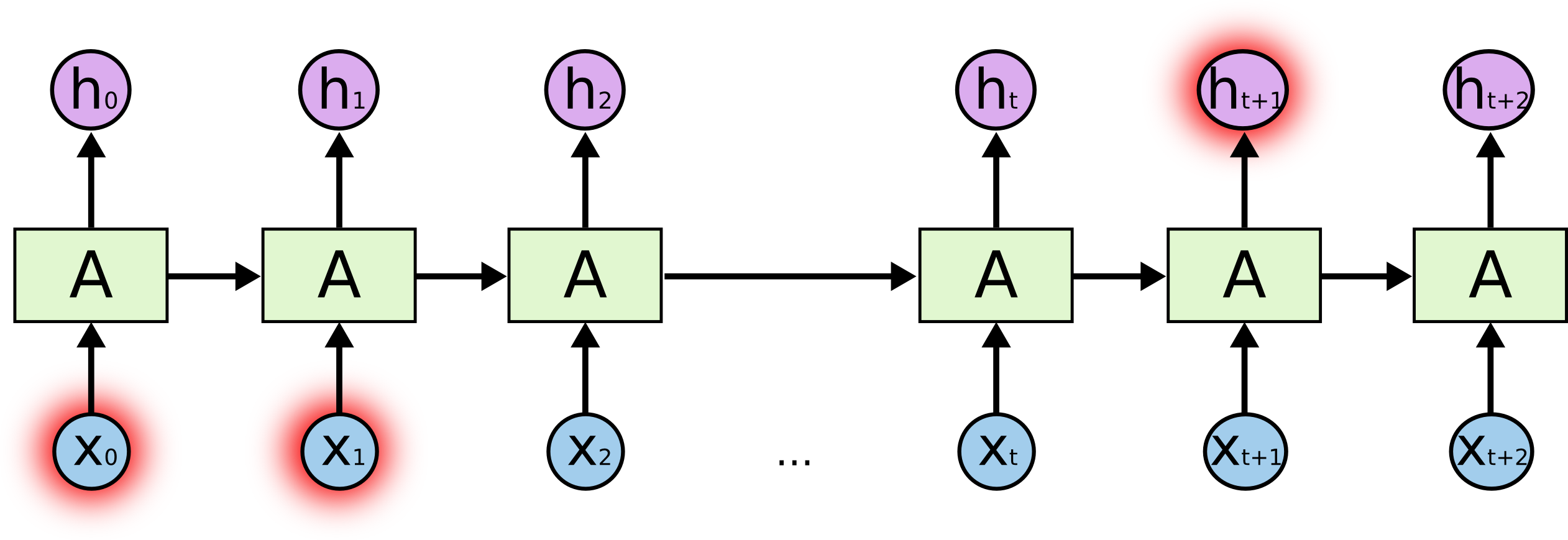
Image Source 3)
RNNs (or CNN) are having a hard time dealing with that since the information needs to be passed at each step and the longer the sequence is, the more likely the information is lost along the sequence. Because when adding a new word to the sequence, all existing information is being transformed by applying a function, effectively modifying what is deemed important in the sequence.
Additionally, recurrent models due to sequential nature (computations focused on the position of symbol in input and output) are not allowing for parallelization in training, this also causes a problem with learning long-term dependencies (Hochreiter & Schmidthuber, 1980) from memory. Naturally, the bigger the memory is, the better, but the memory eventually constrains batching across learning examples for long sequences, and this is why parallelization cannot help.
LSTMs try to solve this problem by introducing cell states. Each cell takes a token as input, the previous cell state and the output of the previous cell. It does some multiplications and additions based on the inputs and generates a new cell state and a new cell output. We will not elaborate on this mechanism since it is out of the scope of this topic.
Up until recently, most approaches used attention with RNNs, however, Transformers are more promising since they allow to eliminate recurrence and convolution and use Attention to handle the long-term dependencies. Additionally, Transformers are easier to parallelize which speeds up training time.
Attention allows Neural Networks to focus on certain parts of a sequence they are given. The intuition behind this is that there might be relevant information in every word in a sentence.
We will elaborate on the Self-Attention process later. First, we will look at the GPT-2 architecture and the way it handles inputs since this is important to understand the inner mechanisms of the Attention process.
GPT-2 Architecture
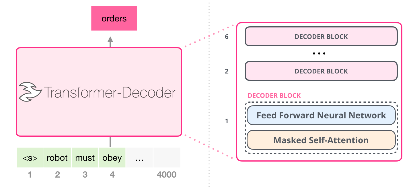
The GPT-2 architecture is no novelty, in its core, it is very similar to the Decoder-only Transformer and GPT-2s earlier iteration GPT (Radford et al., 2018).
GPT-2 is available in different versions regarding the architecture, or rather sizes.
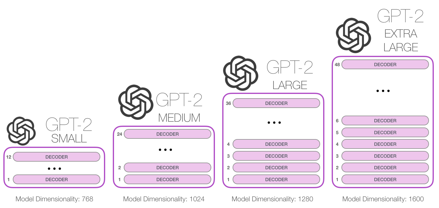
Image Source 4)
We used the smallest version of GPT-2 because of computational and time restrictions with Google Colaboratory. For this project, it made sense to leverage the GPU processing capabilities supported by Google Colaboratory.
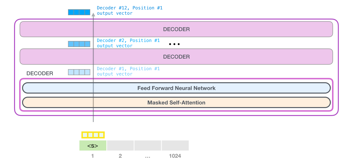
GPT-2 (Small) has 12 Decoder Blocks. Each Decoder block has a Masked Self-Attention layer using 12 attention heads and a dimension size of 768 followed by a two-layered feed-forward Neural Network. It results in 124 million parameters which is still a lot and should allow the model to understand the language characteristics of the input language.
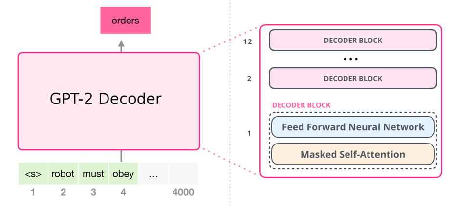
Image Source 5)
The bigger versions of GPT-2 work the same in their inner mechanisms. The only two differences are that the bigger models have a higher model dimensionality and stack more Decoder blocks on top of each other.
The respective code:
How does GPT-2 create text?
On a high level, GPT-2 takes a sequence as input and predicts the next word for that sequence. That word is then added to this input sequence and used for the next prediction. This mechanism is called “auto-regression”. In the follwing explanations, I will use “token” and “word” interchangeably.

Image Source 6)
Input Encoding
To understand how GPT-2 generates text, it makes sense to start with the inputs. As in all other Natural Language Processing models, the text input needs to be encoded since Neural Networks cannot work with raw text data (strings). These models need numerical representations of words to be able to process them.
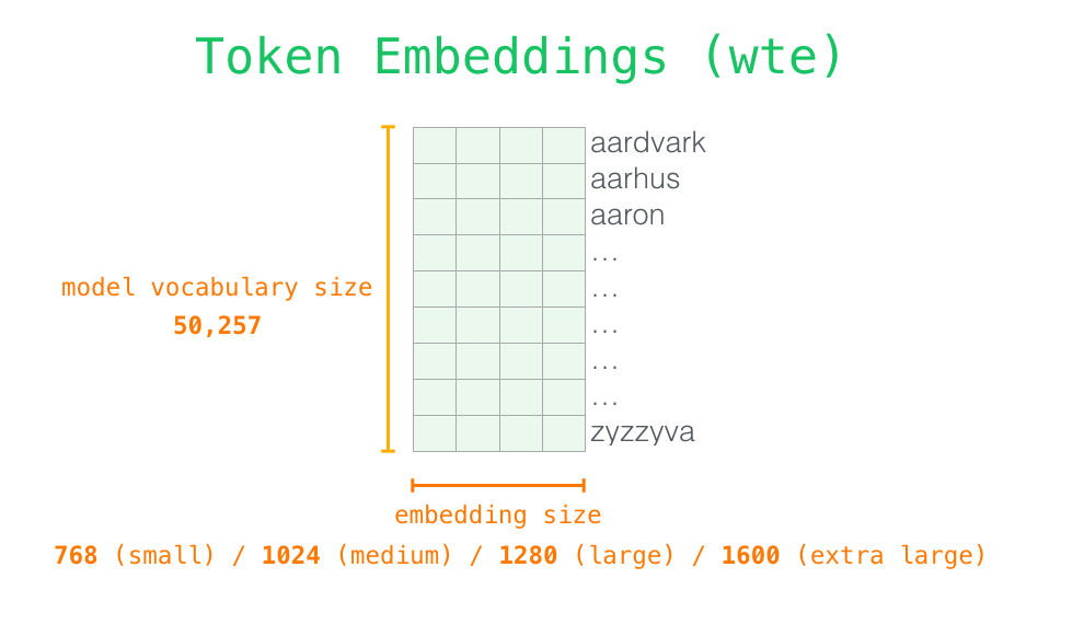
We use Token Embeddings (wte) and Positional Encodings (wpe) to achieve that (Radford et al., 2019).
Token Embeddings (wte)
Each row is a word embedding, basically a numerical representation of this word which captures some of its meaning. The size of the token embedding represents the model dimensionality, in our case 768 (GPT-2 small) for every token.
The respective code:
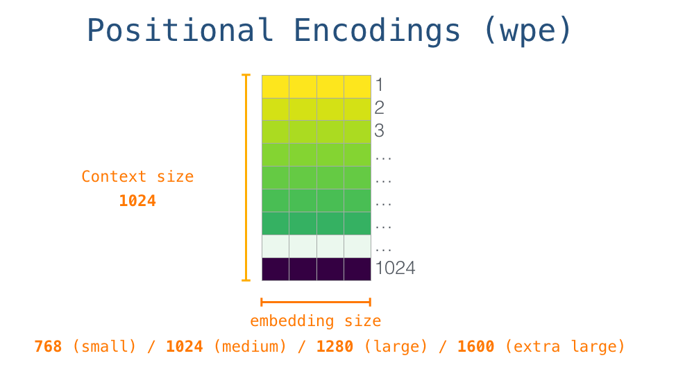
Positional Encoding (wpe)
The positional encoding is an indicator of the position of a token in the sequence. During the pre-training of GPT-2, a positional encoding matrix is learned, the same applies to the token embedding matrix.
The respective code:
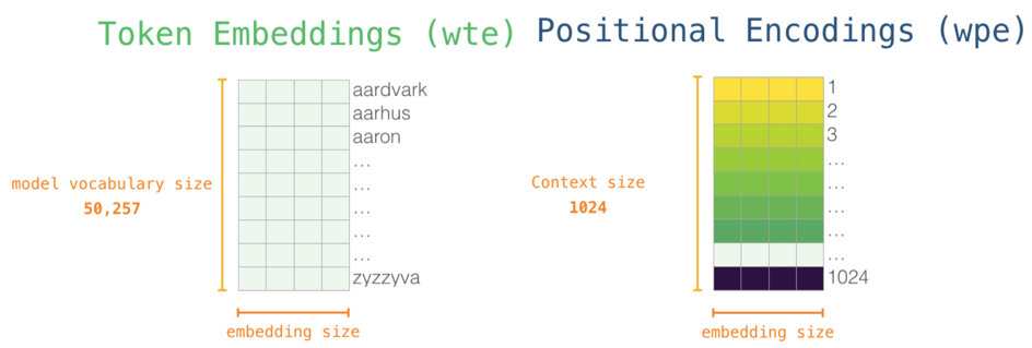
Image Source 7)
The embedding matrix will be handed together with the positional encoding matrix to the Masked Self-Attention layer of our first Decoder block.
GPT-2 - Token Processing Overview
On a high level a token gets processed the following way:
- The token (in reality, it’s the vector in the embedding matrix together with the positional encoding for that token) is handed to the first Decoder Block.
- The Decoder Block passes the token through the Masked Self-Attention Layer and the Feed Forward Neural Network
- The Feed Forward Neural Network sends a result vector up the stack to the next Decoder Block
- The last Decoder Blocks result vector gets scored against the GPT-2 vocabulary
- And finally outputs the token with the highest probability
This process is identical in each Decoder block, but each block has its weights in both self-attention and the Neural Network sublayers.

Image Source 8)
Self-Attention Process
We will explain the whole process on a vector level since it is easier to understand, although GPT-2 is actually using matrices for all the operations in the Self-Attention process.
Query, Key and Value vector
The first step in calculating Self-Attention is to create three vectors for the input word (in this case, the embedding and positional encoding of that word) which is processed at the moment.
So, for each word, we create a query vector, a key vector, and a value vector. These vectors are created by multiplying (dot product) the embedding by the query weight matrix WQ, the key weight matrix WK and the value weight matrix WV that were created during the training process.
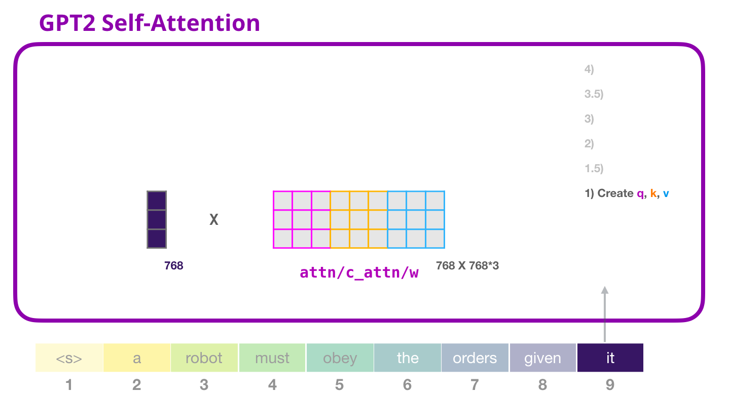
Image Source 9)
Splitting into Attention Heads
We proceed with splitting our query, key and value vectors in such a way that we obtain a matrix with 12 rows and a dimension length of 64 for each of the three vectors. Every row in our new matrix will one attention head.
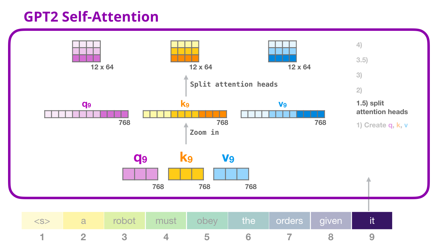
Image Source 10)
This procedure improves the performance of the Attention layer in two ways:
- It expands the model’s ability to focus on different positions. In the example above, it would be useful if we’re processing a sentence like “a robot must obey the orders given it”, we would want to know which word “it” refers to.
- It creates multiple representation subspaces. As we’ll see next, with multi-headed Attention we have multiple sets of Query/Key/Value weight matrices (GPT-2 uses 12 attention heads, so we end up with 12 sets for each decoder block). Each of these sets is randomly initialized. Then, after training, each set is used to project the input embeddings (+ positional encoding) or vectors from lower decoders into a different representation subspace.
Scoring
In the second step, we need to score each key vector of the other words in the input sentence against the query vector of the word we are processing at that moment.
The score is calculated by taking the dot product of the query vector with the key vector of the respective word we’re scoring. So if we’re processing the self-attention for the word in position #1, the first score would be the dot product of q1 and k1. The second score would be the dot product of q1 and k2. This is done for every of the 12 attention heads.
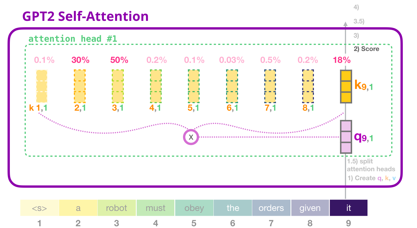
Image Source 11)
The score impacts how much focus to place on other parts of the input sentence as we encode a word at a certain position.
The third and fourth steps are to divide the scores from the dot product of query and key vector by the square root of the dimension length dk of the key or query matrix, which is 64 and thus effectively dividing by 8. This leads to having more stable gradients. We recall, that the dimension length is 64 because our embedding size is 768 for GPT-2 small and thus the size of our key and query vector is 768, we proceeded with splitting these vectors into 12 attention heads resulting in 12x64 matrx.
We pass the result through a softmax function. Softmax normalizes the scores so they are all positive and add up to 1. This softmax score regulates how important each word will be in this position.
In the fifth step we multiply each value vector by the softmax score we just calculated. The idea here is to keep intact the values of the word(s) we want to focus on and minimize the impact of irrelevant words (by multiplying them by small numbers like 0.001, for example).
The formula looks as follwing:
$Attention(Q,K,V) = softmax(\frac{QK^{T}}{\sqrt{d_{K}}})\ V$
The respective code for steps two to five is:
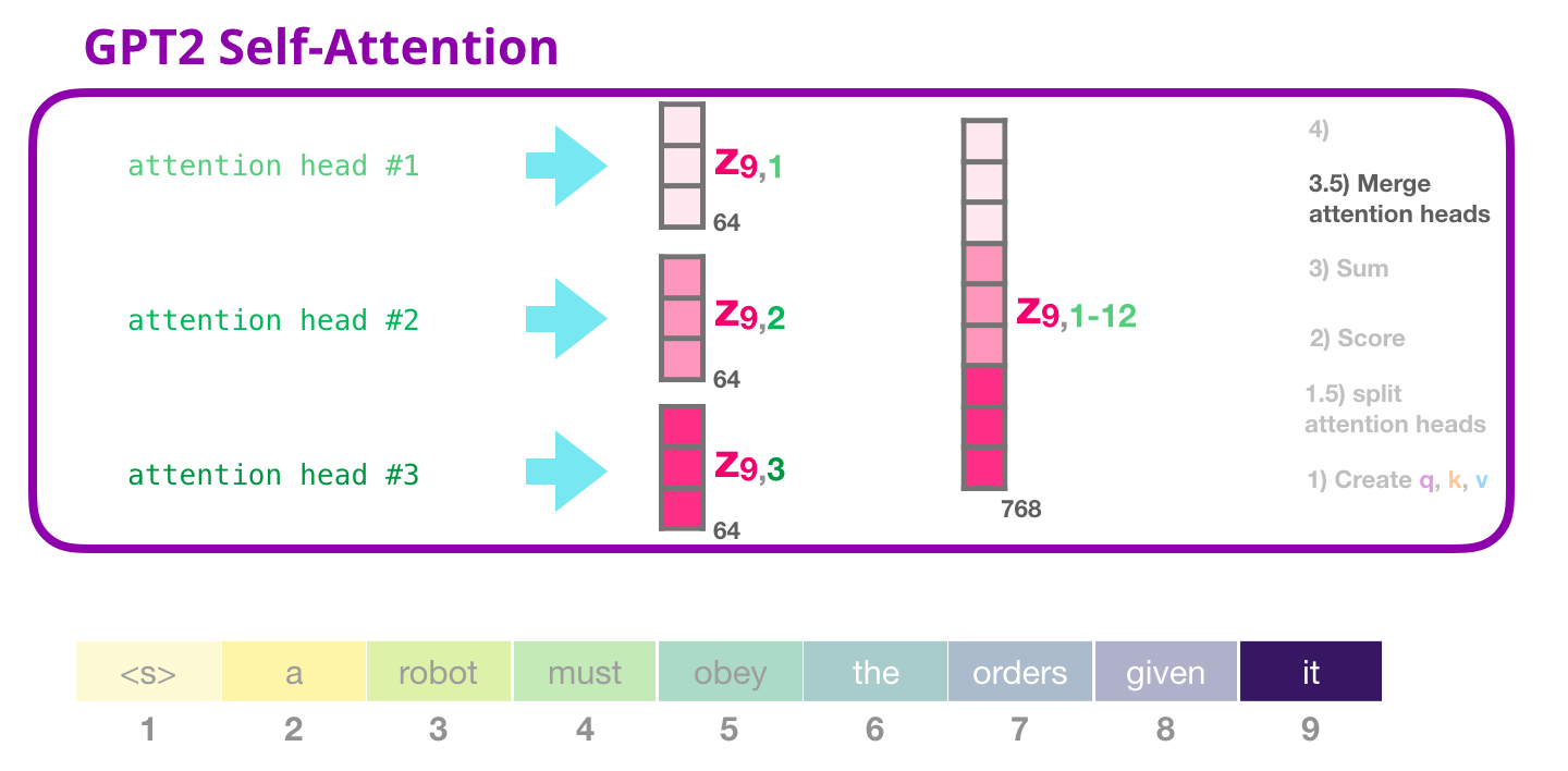
Sum
The sixth step is, to aggregate the weighted value vectors, producing the result vector of the self-attention process for an attention head. We do the same self-attention calculation we explained above, just 12 times with different weight matrices which results in 12 different Z vectors. Since the feed-forward Neural Network is expecting a single vector (matrix) as input (a vector for each token), we merge the resulting vectors of the 12 attention heads into a single vector.

Image Source 12)
The resulting vector is still not ready to be feed to the following Neural Network and thus we multiply (dot product) it with yet another weight matrix (learned while training). This transforms the results of the 12 attention heads to the output vector of the Self-Attention layer which can be sent to the Feed-Forward Neural Network.
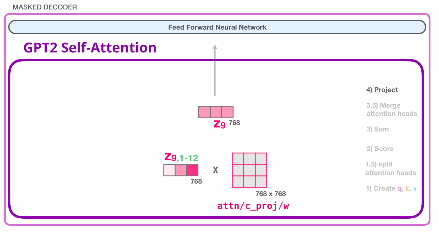
Image Source 13)
The respective code:
Although the whole Self-Attention process should be clear by now, what is the result vector of the Self-Attention layer doing?
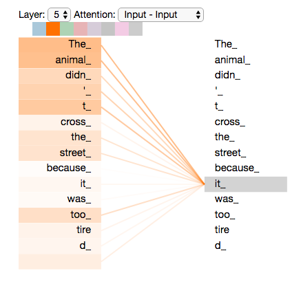
The following example should clarify that:
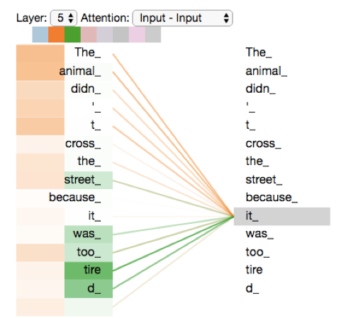
Image Source 14)
As we process the word “it”, one attention head is focusing most on “The” and “animal”, while another is focusing on “tired”.
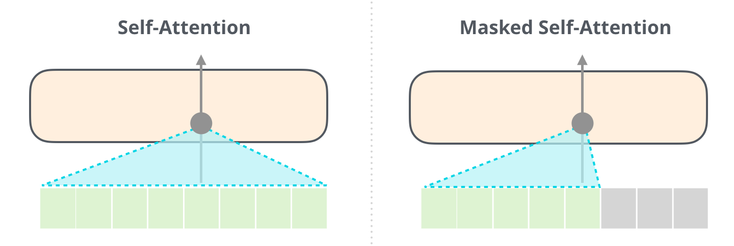
This was the whole Self-Attention process. There is still a little detail which we left out on purpose, GPT-2 uses Masked Self-Attention and not Self-Attention. So, what is the difference?
Masked Self-Attention
Masked Self-Attention is almost identical to Self-Attention, the only difference is in the scoring step. The inputs in the sequence which are right from the current position are not considered.
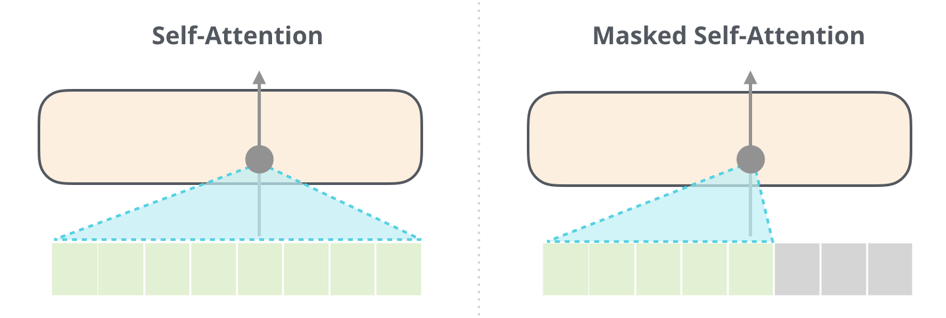
Image Source 15)
The respective code:
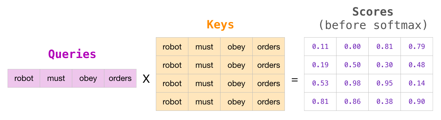
Let us look at the following example:
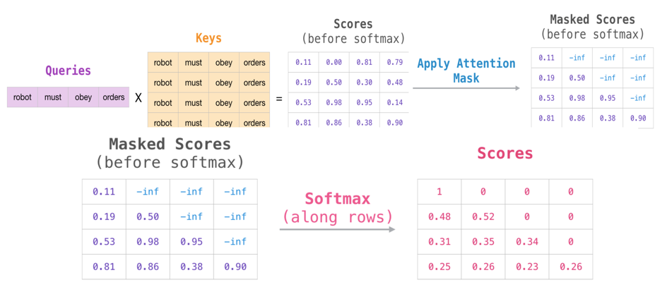
Image Source 16)
We consider an input sequence of 4 words. The Query vector of each word is multiplied (dot product) by the Key vector of each word in that input sequence. This results in an intermediate score, which again gets divided by the square root of the dimension length to produce the “Scores (before softmax)”.
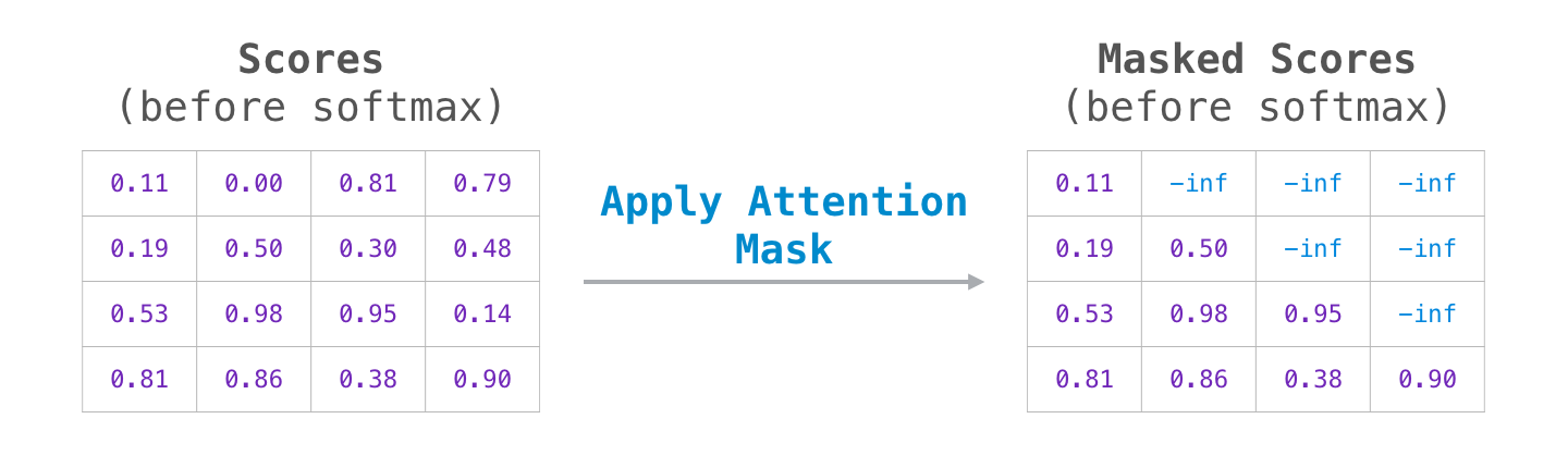
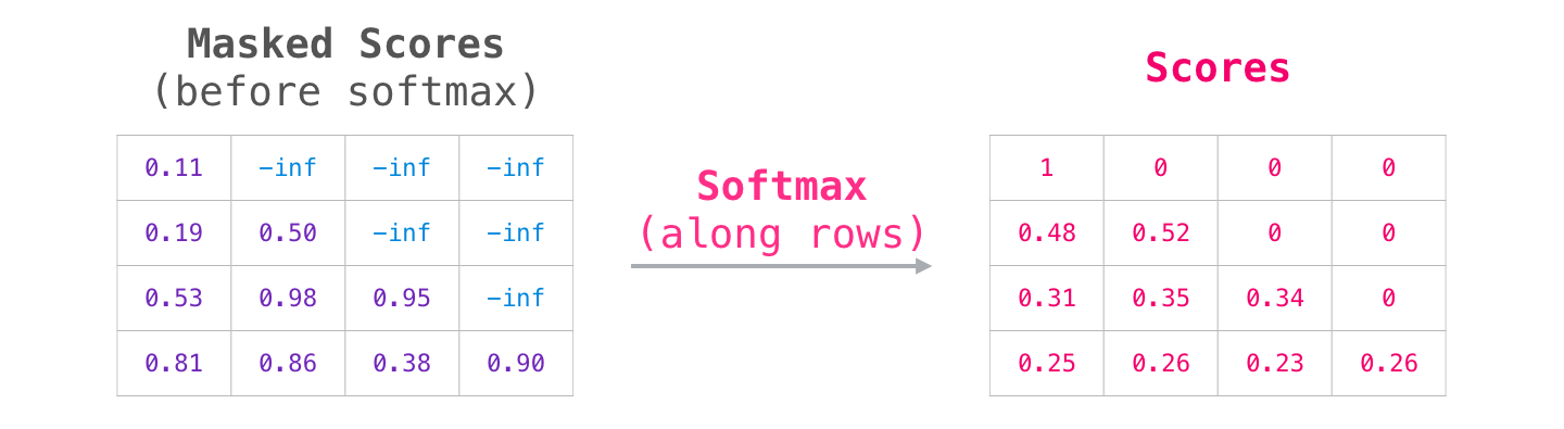
We apply masking using a matrix in which the scores to the right of the current position get a large negative number. Applying softmax on each score produces the actual scores used in Self-Attention.
The last table with the final scores is to be interpreted as follows:
- When processing the first row, representing the word “robot”, 100% of the attention will be on that word.
- When processing the second row, representing “robot must” and it processes the word “must”, 48% of its attention is on “robot”, and 52% on “must”
This continues with the same logic.
Feed-Forward Neural Network
As mentioned above the result vector of the Masked-Self-Attention layer gets handed to the Feed-Forward Neural Network which has two layers.

Image Source 17)
As in any other Neural Network inputs get multiplied by some weights. In this case the input is the resulting self-attention vector which is multiplied (dot product) with the weight matrix of the first Neural Network layer.
The second layer transforms the result of the first layer back into a vector of dimension length 768 which can be processed by the next Decoder block up the stack.
Image Source 18)
The whole procedure starts again but with other weights for the Self-Attention layer and the Feed-Forward Neural Networks of our next Decoder blocks.
The respective code:
This cycle ends with the last Decoder block in the stack, for GPT-2 small this would be the 12th Decoder block.
Model Output
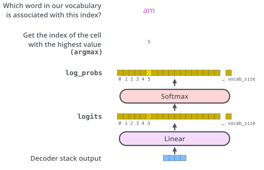
The top Decoder block outputs the final result vector of the Masked Self-Attention process and its Neural Network, how do we get an output word out of it?
In the final Linear layer our final result vector is projected into a logit vector using the word embeddings wte (we multiply (dot product) our result vector with the embedding matrix). This logit vector consists of logit scores for every word in our model´s vocabulary (about 50k words for GPT-2).
The Softmax layer transforms these scores into probabilities and our model outputs the word which is associated with the highest score in this probability vector.
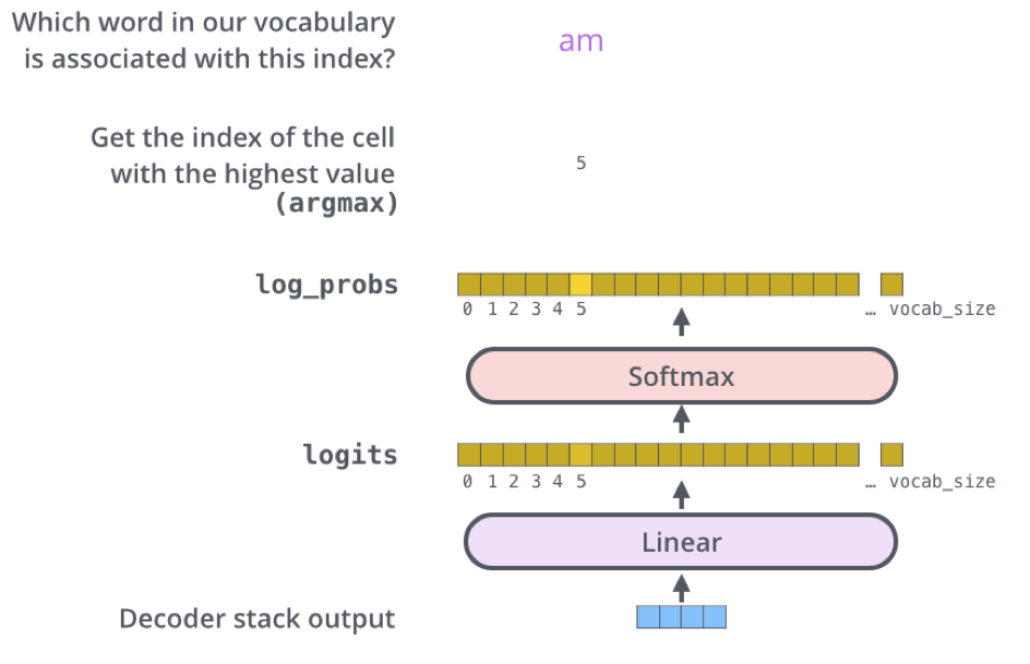
Image Source 19)
The respective code:
Byte Pair Encoding
Byte Pair Encoding - Introduction
In this section we aim to explain why GPT-2 is able to recognize German words, although trained solely on English text data from the web. To understand why GPT-2 can be used to generate German text, it is necessary to understand the functioning of byte pair encoding (BPE) in NLP.
Originally, BPE was developed in 1994 by Philip Gage, as a comparatively simple form of data compression. The main idea was to replace the most common pair of consecutive bytes in a data file with another byte, which does not belong to the set of occurring characters. Thus, the BPE-algorithm checks the whole text corpus for multiple occurrences of character-/(byte-)pairs and converts them to another character/byte. Thereby, the size of the original data is compressed by reducing the amount of characters that is necessary to represent that data. In order to decompress/decode the compressed/encoded data again, it is necessary to provide a table of executed replacements. This table allows to rebuild the original data by mapping the replacement characters back to their original representations (character pairs). The original and the decompressed data should be equal at the end, to ensure consistency.
Hence, BPE allows to reduce the length of character sequences by iterating through the text corpus several times. The algorithm can reduce the size of the data as long as a consecutive byte pair occurs at least two times. Since BPE is a recursive approach, it allows further to replace also multiple occurrences of replacement character pairs. This can be used to even encode longer sequences than only two bytes with only a single replacement character. Although the BPE-algorithm is not the most efficient form of data compression, it offers some valuable aspects for the use in NLP.
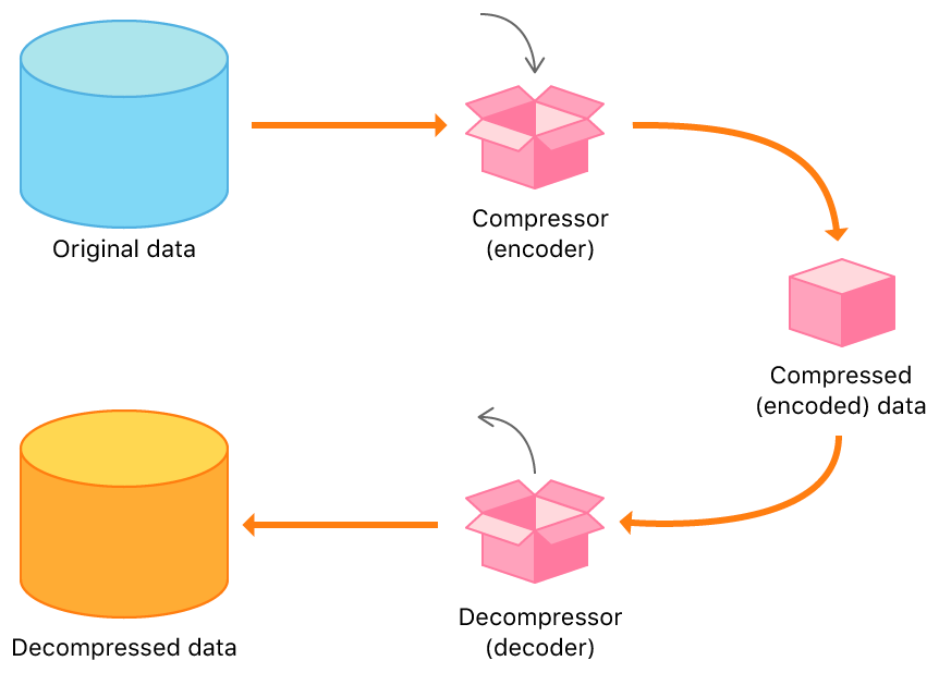
Image Source 20)
Byte Pair Encoding for NLP
The idea of BPE can be repurposed for the use in NLP applications. One main aspect in this regard is the reduction of the vocabulary size. To achive this, the original BPE algorithm needs to be modified for the use on natural language text. The reduction of the vocabulary size is realized by using a subword tokenization procedure, which is inspired by BPE.
In general, there are three levels, in which words can be included into a vocabulary (see figure below). The first is the word level representation where only complete words are used in the embedding. For each word, a vector is calculated to capture its semantics. This generally leads to large embeddings, depending on the amount of text and heterogeneity of words included. The second option for determining vector representations of words inside an embedding is to reduce words to character level. This significantly reduces the size of the vocabulary since only the set of contained characters is left. However, the usage of character level word representations in NLP resulted in comparatively poor outcomes in some applications as shown e.g. in Bojanowski et al. (2015). The third option is to use subwords instead of character or word level representations. This offers a good balance between both previous types of word representations by combining the advantages of a reduced vocabulary size with a more “meaning-preserving” word splitting.
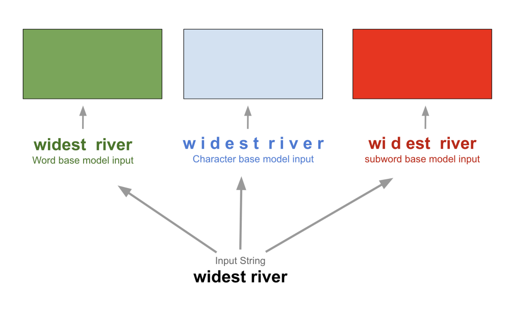
Image Source 21)
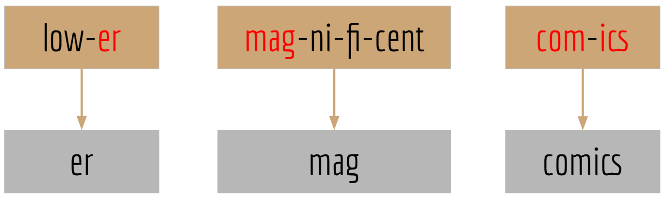
Additionally to the reduction of vocabulary size, there are several more advantages of splitting words into subwords. These are primarily important for our application, i.e. the generation of German text by using an “English”-language model (GPT-2). First, the language model does not fall into out-of-vocabulary-error, when a German word is presented to it. Words from the German vocabulary can be perceived as unknown to the vocabulary of the English language model. Although GPT-2 was not provided with German text during training, there exists a number of subwords that are equal in German and English. An example is given in the figure below. Since single characters are also included into the GPT-2 vocabulary, German words that cannot be constructed out of multi-character subwords are simply represented at single-character level.
Another useful advantage of splitting words into subword tokens, is the fact that rare words can potentially be returned in the output of the generation process. When using word level embeddings for a large text corpus, it is generally necessary to reduce the vocabulary size by setting a fixed limit to the number of words. This means that very rare words, that only occur e.g. one or two times in the whole corpus, drop out of the set of words that can appear in the generated text. By splitting rare words into much more frequent subwords, these can still be included in the resulting synthetic text.
A major modification that is necessary to use BPE in NLP applications is that pairs of subwords (bytes) are not replaced by another character, but rather are merged together to a new subword. This is done for all instances of a pair in the whole text. The process can be repeated as long as all words are broken down into segments. Therefore, the subwords that are included in the resulting vocabulary are dependent on the underlying text corpus. The GPT-2 vocabulary consists of approximately 50.000 subword tokens. It is possible to set certain parameter values that limit the merging of subword pairs, depending on their frequency of occurrence. The NLP-adapted BPE algorithm does not fulfill the original task of data compression, since it does not reduce the amount of raw data. It rather represents a splitting heuristic that is able to adjust the subword vocabulary to the text it is applied to.
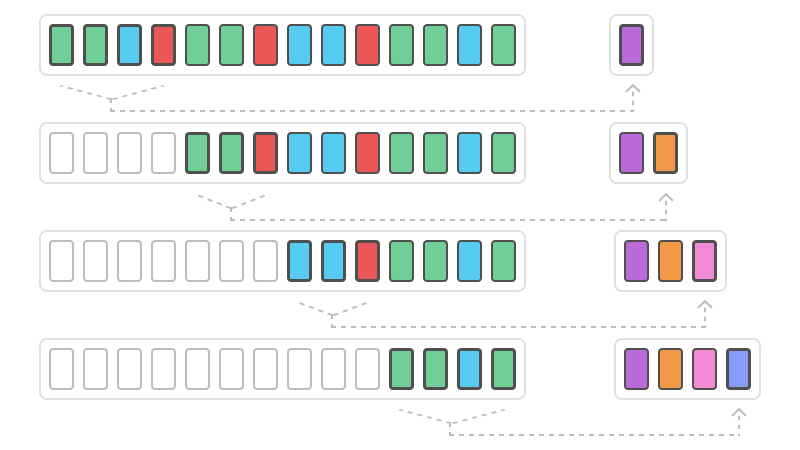
Image Source 22)
The BPE-based subword tokenization helps us to explain, why German words are part of the GPT-2 vocabulary and does not lead to an out-of-vocabulary error. However, since the meaning of subword tokens are in most cases completely different across both languages, it cannot be explained how pre-trained language information from GPT-2 can be transferred to our German text generation process. It is not even clear whether any semantical or gramatical knowledge is transferred at all. For example, the German word “die” as female article and the English verb “(to) die” have a completely different meaning. Therefore, the pre-trained word vectors from GPT-2 are expected to be more or less useless to capture the meaning of German subwords from our comment texts (although exceptions exist, e.g. alphabet, film, hotel). That means that the majority of knowledge about grammatical and semantical dependencies of the German language has to be learned during the fine-tuning of the GPT-2 model.
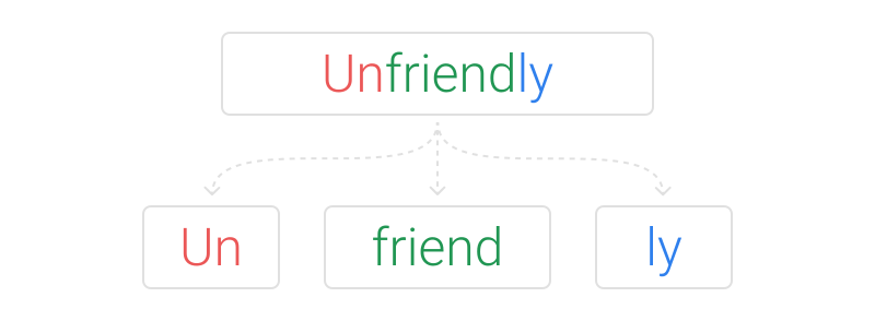
Image Source 23)
Comparing Generated Text
When comparing the comments generated with the first Language Model with those generated with GPT-2, it is noticeable that GPT-2 performance significantly better. The following table shows examples of good and bad generated comments.

Comment Classification Task
Relation to Business Case
In our business application scenario above, we described that a large number of employees is necessary if we want to check each incoming comment manually. Due to legal regulations and business compliance goals, there is no opportunity to not check every individual comment.
Our aim is to tackle this issue by training a classification model on existing comments that were already manually labeled as publishable or not. The model should be capable to differentiate between comments that violate any of the given restrictions, and those that do not. This leads us to a binary classification setting, in which we want to predict a probability of being publishable for each comment.
Classification Approach
In our classification stage, we train several models on different data inputs. With the resulting probability predictions, we can decide how to deal with the comment and evaluate the model performance. Since our data is imbalanced with a ratio of approx. 85:15 (majority class: published comments), we face different classification settings that are explained below. We further use two different classifiers in our application to allow for a comparison of the results among different classification approaches. The architectures of the two classifiers is described in the following.
Classification Architecture
RNN Classifier
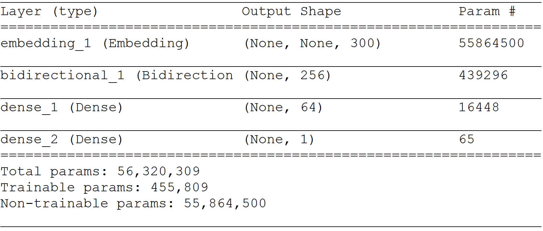
For our binary classification problem, we first construct a recurrent neural network (RNN), of which the model architecture is depicted below. We include an embedding layer into our model, which uses a Word2Vec embedding that we trained on 1 million comments from our own text corpus. We further included a bidirectional LSTM Layer in our model to capture the sequential character of our data. To obtain the required output from our RNN model, we include two dense layers. The first uses relu and the second sigmoid as activation function. The second dense layer turns our values into the required output format, i.e. a probability prediction for each comment.
BOW - Logistic Regression-Classifier
Additionally to our RNN-classifier, we train a comparatively simple Bag-of-Words (BOW) Classification model, which uses logistic regression to predict the probability for a comment to be publishable. This second model is also trained with the same data composition/distribution as the RNN-model, in each of the four classification scenarios. The second classifier serves as a benchmark model to evaluate the performance of our RNN-model, in each of the classification settings. Although a comparatively simple approach, the combination of BOW and logistic regression has shown to yield at good results in similar applications (see e.g. Sriram et al., 2010).
Classification Settings
The classification settings vary in terms of the data we input to our two models. Since our main goal is to examine the use of generated comments to balance textual data, we need a benchmark to measure the impact of our synthetic comments. In total we end up with four different classification settings, that can be divided into either benchmark (imbalanced, undersampling) or target (both settings including generated comment data).
We use both our classifiers in each of the settings that are described in the following part. For the first setting (Imbalanced) an extended explanation of the code is given below to describe our classification approach more in depth. Since the classification architecture is equal for all settings, we do not describe the code for the reamining ones. However, we will give code examples for the data preparation that varies for the other settings.
(1) Imbalanced
In the imbalanced setting, we use the cleaned comment text data to train our models. Hence, the classifiers are provided with the imbalanced comment data from the original data set. We did not change the distribution of publishable and non-publishable comments. The imbalanced setting is meant to serve as a first benchmark for our following classification settings.
The implementation of the Bag of Words (BOW) Classifier is constructed as shown in the code below. We first count word occurrences using the CountVectorizer from the scikit-learn package. Next, we run a logistic regression to estimate the relations between word occurrences and the publishing status of our comments. The ‘bow_classification’-function returns the predicted probabilities of being published for the comments in the test data.
For each model in all of our settings we calculate evaluation metrics based on our model predictions. We convert our probabilities to class predictions, using a threshold of 0.5. Next, we build a confusion matrix for each model using the pandas crosstab function. These confusion matrices are used during the evaluation phase to compare the models accross settings.
Furthermore, we are able to calculate additional metrics that allow us to evaluate the performance of our binary classification models. We use sklearn.metrics functions to determine F1-Score, the area under receiver operating characteristics (ROC) curve (AUC) and the accuracy of our predictions.
For the recurrent neural network classifier (RNN), some additional preparation steps are neccessary to fit the model. First, we perform tokenization using the text tokenizer from keras text preprocessing. Second, we are padding the sequences to a fixed length, which we set to 100.
After preparing the data, we configure our RNN classifier. Therefore, we first set our parameter values. Since they have to be equal for each setting, it is practical to set them globally at a fixed position in the code.
Afterwards, we configure our model architecture, which was already described in the previos section. We use keras for our RNN implementation. As optimizer for the model we take the adam optimizer and since our target task is a binary classification, we use binary crossentropy for loss minimization.
After training the RNN model, we predict class probabilities for our test data. Similar to the BOW model case, we calculate the confusion matrix and our evaluation metrics for the RNN model.
(2) Undersampling
The second benchmark setting of our classification part consists of a simple undersampling approach. We reduce the number of comments from our majority class (published comments) to balance our data set. Since our data is imbalanced with a ratio of 85:15, we need to exclude a significant amount of published comments, in order to align them to our minority class (not published comments). Obviously, the disadvantage in this setting is that we hide available information from our classifiers, that might contain useful information to identify publishable comments. We use this setting as a second benchmark because, in contrast to our imbalanced setting, we now have a balanced situation that we want to achieve also in our target settings by including synthetic comments.
Both our benchmark settings are useful to evaluate the impact of our generated comments on the outcome of the classification. The imbalanced case allows us to compare the outcomes between an imbalanced and a balanced text classification task. The amount of original data is not changed but the distribution of both classes is different. The undersampling scenario is used to compare the outcomes of classification tasks provided with a balanced data set. Here, we change the amount of original comments by reducing the number of observations from the majority class. Thus, the distribution of both classes is balanced.
(3) Oversampling GloVe
In both our oversampling scenarios (GloVe and GPT-2), we use synthetic comments of our underrepresented class (not published comments) to balance our comment type distribution. The advantage of this approach is that we can use all of the available original text data for the classification. In contrast to the undersampling case, we do not need to exclude any comments, but still reach a situation where we have a balanced distribution of published and unpublished comments. Hence, we provide our classifiers with both, the original data and the synthetic comments that were generated by using the pre-trained German GloVe embedding.
The generated text data is also edited using the cleaning function for classification from above. Then we extend the original data with the synthetic comments of the underrepresented class (not published) and the according label for the publishing status.
(4) Oversampling GPT-2
Our second oversampling scenario is conceptionally equal to the first one. The only change in this scenario is the use of the pre-trained GPT-2 language model for the creation of synthetic comments instead of the GloVe-based generation architecture. A major difference between GPT-2 and GloVe in our application is that they were trained on text data of different languages. GPT-2 was trained on massive amounts of English text data. It has advanced capabilities in the generation of English text by fine-tuning it to domain specific textual data. We want to make use of this generative power of GPT-2, but since our data set consist solely of German text, we face a severe drawback regarding the language-related barrier. On the other hand, the GloVe embedding we use was trained on German text only. Therefore, we do not need to overcome the language differences. However, text generation with using a GloVe embedding might not have the same generative power as GPT-2. Thus, we have a trade-off between language-related differences and the generative capabilities of both generation approaches.
Drawbacks of Oversampling with Generated Text
The balancing of textual data using generated text is based on the simple concept of adding synthetic comments of the underrepresented class with the corresponding label to our data. Since only non-publishable comments are taken as input for the generation models, our resulting generated text is expected to imitate only that type of comments. This is an assumption we make and since this is an essential point for our approach, we want to discuss it here in more detail.
The comment data that we use for the text generation is probably noisy. We are not always able to explain why a comment has been banned from the comment section. Some comments might be labelled as non-publishable without any justification. For example, comments are marked as “not-published” before they were checked. There is a high probability that a comment, that was not manually verified so far, will be published after it was checked. Other comments might also be simply banned due to an erroneous assessment by an employee. There are legal and company-provided guidelines for the comment assessment. In some cases, the decision might differ due to the perception or interpretation of an employee that reads the comment. A comment that is at the boundary between being publishable and not being publishable, might be classified differently by different employees that check it.
If this kind of noise is included in our data, then we reproduce the noise by generating comments based on that noisy text. By including the generated comments in our classification training phase, we increase the noisy data the classifier must deal with. Hence, it might become increasingly hard for the classifier to differentiate between both comment types.
Classification Task - Limitations
There are some limitations to our classification approach that we want to point out here.
First, we use only the cleaned and tokenized text as an input for both our classifiers. Meta-information about the comments, like the number of words included or the date when a comment was created, are not taken into account.
Second, due to the fact that the text generation takes a significant amount of time by using our limited computational resources, we are not able to use all our available real comment data to train the models. We reduce the amount of comments in our training set depending on the available amount of synthetic comments.
Third, the usage of generated comments to balance our dataset inserts noise into our training data. The amount of noise is thereby highly dependent on the number of comments that are used as “original examples” for the generation models and also on the ratio of real and synthetic comments in the minority class. When only a very small number of text examples is available for the text generation, then the resulting synthetic comments might be too homogenous to serve as meaningful input for the classifier. Further, if there are only very few real comments and a lot of generated ones in the training data, then the inserted noise might confuse the classifier.
Evaluation
For the evaluation of our classifiers across the different settings, we use three metrics: F1-Score, the AUC and accuracy (ACC). Additionally we measure the performance of our models by examining the distribution of predictions. Therefore, we compare our results by the percentages of true/false positive and true/false negative class predictions. These values offer insights into the prediction behaviour of our classifiers.
We are not able to evaluate the results including our third class “not sure”, because we have no ground truth available to check for the correctness of our predictions. The only possibility would be to look at those comments and try to assess whether they are indeed “ambiguous”. An example for the implementation and evaluation of the “not sure”-class is shown later on.
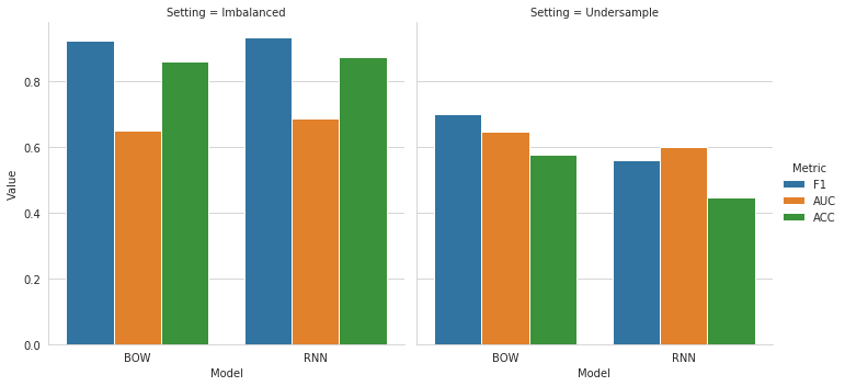
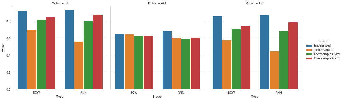
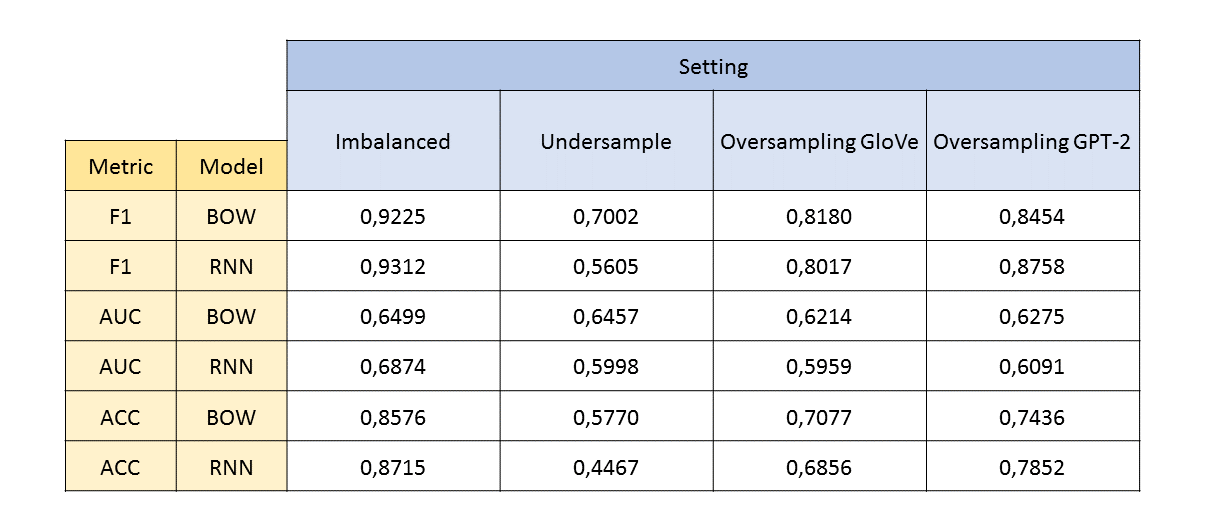
The results are presented below, starting with the evlaution in terms of F1, AUC and ACC. We can observe that for both our baseline settings (Imbalanced and Undersample), the results are better for each metric in the Imbalanced case compared to the Undersampling setting. The results between the BOW and the RNN model are very similar in the Imbalanced scenario. In the Undersampling setting, we observe that the RNN model performs constantly worse than the BOW model, probably due to the small number of comments in the training set.
For the two Oversampling settings, the results indicate a better performance for the models that were trained on generated text based on GPT-2 compared to the models from the GloVe setting. The results in both Oversampling scenarios are also constantly better compared to the Undersampling setting. However, if we compare our model performance from both balanced settings with generated comments with those from the Imbalanced case, we can observe that the results of both Imbalanced models are better for all of our metrics. This clearly indicates that the generated comments do not positively influence the performance of our classification models.
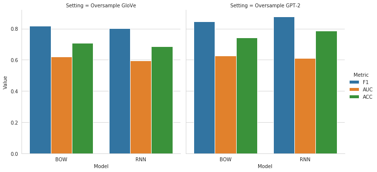
This becomes even more clear if we look at the direct comparison of our metrics ordered by the setting. We can observe that the blue bar, representing the Imbalanced setting, is above the others for all three metrics. The AUC values for our BOW-models are very similar across all settings. But we can also see that the AUC of the Imbalanced setting is slightly above those of the others.
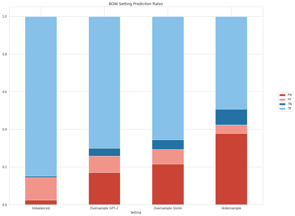
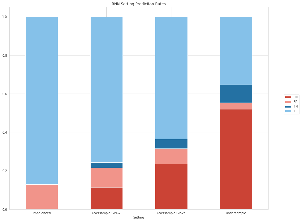
We further analyzed the distribution of class predictions and compare them to their corresponding true value. We use the confusion matrix of each model to extract the true/false-positives (TP, FP) and negatives (TN, FN).
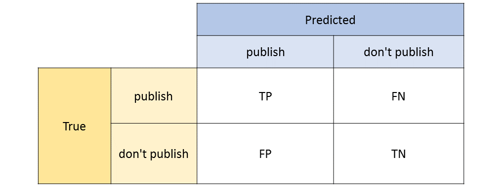
We included 50000 observations (i.e. real comments) in our test set. In the chart below, the percentages for the four prediction cartegories are visualized. The “false” class predictions are represented in red and the “true” ones in blue. We can see that the Imbalanced setting again yielded at the most true values (TP, TN) compared to the other scenarios. Regarding our business case, the class we want to identify most are the negatives, i.e. the comments that are not publishable. Therefore, we want to minimize especially the amount of FP-predictions, i.e. the comments that are not publishable but are classified as publishable. The percentage of correctly classified values (TP+TN) is higest in the Imbalanced setting. However, the percentage of FP and TN are minimal in the Undersampling setting. A severe drawback in the Undersampling case is that we observe a very high rate of FN, meaning that there are a lot of comments that are actually publishable but are clasified as not publishable by the classifier. This means that a large amount of comments would not be published without any justification.
There are some differences between the BOW and the RNN model, especially with regard to the Imbalanced setting. There, we observe that almost all comments are predicted to be publishable by the RNN model. This means that our RNN classifier is highly affected by the imbalanced distribution of comments. This situation is not observed in the remaining (balanced) settings, although the performance in the Undersampling case is very weak. This indicated that we are able to influence the predictions of our RNN model by using our generated comments.
The predictions of the two Oversampling settings lie inbetween the others (Imbalanced and Undersampling). As already observed before, the setting including the GloVe-based generated comments performed a bit worse than the GPT-2 scenario.
 |
 |
Including the “Not-Sure”-Category
As described in our business case at the beginning, we include a “not-sure”-category for comments, for which the classifier does not return predictions with a clear tendency towards a certain publishing status. These comments should be checked manually again by human employees to find a definitive decision. Therefore, the predictions of all models for the comments in the test data set where stored together in a dataframe. To determine which comments should belong to the “not-sure”-class, it is necessary to specify a lower (e.g. 0.4) and an upper (e.g. 0.6) probability threshold. Comments, for which the predicted a probability that lies within the range between these two thresholds, are then regarded as “not-sure”.
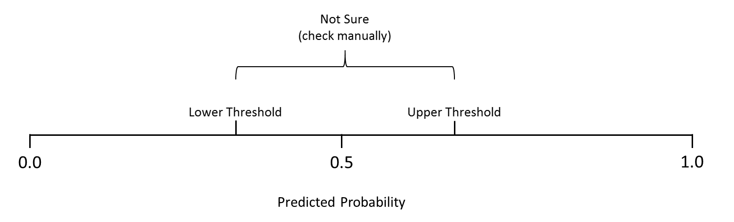
The advantage of specifying an ambiguity range compared to setting a fixed probability threshold (of e.g. 0.5) is that comments for which the classifier could not find a clear tendency will be checked again by an employee. Assuming that the classification returns reliable probabilities, comments that lie around 0.5 can be perceived as difficult to assess. By doublechecking these comments manually by an employee, the final decision about whether a comment violates given legal and/or compliance restrictions, will be supported by human assessment. However, this assumes that our classifier is able to determine the publishing status with a high level of correctness. This is necessary to ensure that comments which are outside the ambiguity range indeed belong to the corresponding class.
By manually checking comments with an ambiguous class prediction, we are able to evaluate the classification performance from another point of view. Since comments that are marked as “not-sure” are manually checked again anyway, we can exclude them from the test set and repeat the evaluation with the remaining comments. The target is to assess the classifier performance only for comments where a clear tendency with respect to the publishing status was predicted.
In the code below, we implemented the steps for including a “not-sure”-category. Therefore, we picked only one example setting (Oversampling GPT-2), since it works equally for the other predictions. As shown in the code below, we first set the two thresholds and then we identified the indices of comments with a probability prediction within that range. Afterwards, we construct a new Data Frame without these identified comments. To compare the results with those including all comments, we calculate again F1-Score, AUC and accuracy as well as the resulting confusion matrix.
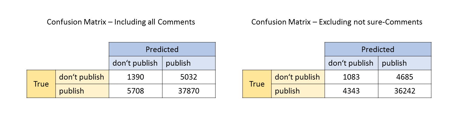
We can see in the table below that the results are better in terms of the F1-Score and the Accuracy. However the AUC is significantly worse when excluding the “not-sure” comments. The reason for that becomes clear if we take a look at the two confusion tables.
Table not sure metrics
A big share of the TN (don’t publish) observations are removed when including the “not-sure”-categroy. This has a negative impact on the AUC. Furthermore, that means that many comments that are predicted to be not pubishable, have an ambiguous probability score.
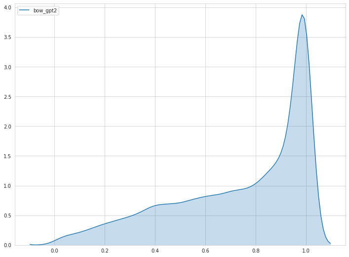
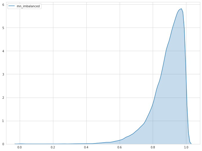
There are also severe differences between the impact of including a “not-sure”-class among the different models. The amount of comments which are labeled as “not sure”, heavily depend on the model predictions. When looking at the distributions of the probability predictions of different models, we can recognize severe differences. The curves below represent the probability distributions for the BOW model in the Oversampling GPT-2 setting and the RNN model in the Imbalanced setting. We can clearly see that in the GPT-2 setting, the BOW model predicts probabilities more distributed over the probability range. Therefore, more comments are labelled as not sure. The RNN model from the Imbalanced setting on the other hand, predicts a probability close to 1 for most of the comments.
Depending on the probability distribution, it is possible to adjust the threshold depending on the given percentage of comments that can be checked manually. In this case, approx. 7.5% of the comments from the test set were labelled as “not sure” (range: 0.4-0.6). When more resources are available to check comments manually, then the range could be extended to include more comments into the “not sure”-class.
 |
 |
Different Balancing Ratios for Generated Comments
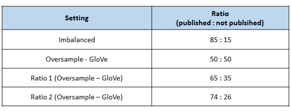
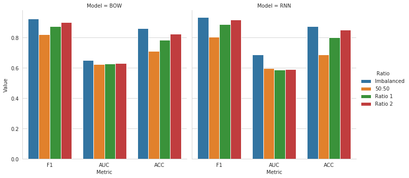
As already stated earlier, using generated comments to balance text data comes with the drawback of inserting noise into the oversampled class of text. In the previous settings where we used generated comments (Oversampling GloVe/GPT-2), we included that amount of synthetic comments of the underrepresented class (not pubished), that yielded approx. at a 50:50 – balancing ratio. To test whether the ratio has an impact on the results, we repeat the classification model training again with different ratios of published and not published comments. We try two additional balancing ratios by iteratively reducing the number of synthetic comments. Afterwards, we compare the results of these two modified settings with the results of the Imbalanced setting, where we include no generated comments and the 50:50-balancing ratio setting. The different ratios are described in the table below.
The results show that the usage of synthetic comments negatively influences the model performance. We can see that the results are best in the Imbalanced setting. The results improve if the ratio of comment classes gets closer to this from the imbalanced one of the original data. It seems that our generated comments insert too much noise and therefore cause a worse performance of the classification models.
Conclusion and Discussion of Results
The evaluation of our results allowed us to assess the performance of our various models across settings. We aimed at improving text classification results by balancing text data with generated comments of the underrepresented class. The results do not support our hopethesis, that the intrusion of synthetic text improves our classification results. We observed that the utilization of genreated comments yielded at better results compared to the Undersample setting. However, the best results were produced by using the original imbalanced comment data. The results from the two Oversample settings were expected to be at least not worse than those from the Imbalanced.
There might be various reasons why we observed the final outcome. First, the intrusion of noise through using generated comments might overweight the potential advantages of training the models with a balanced dataset. Second, the change of the distribution of published and not published comments leads to higher numbers of minority class predictions. This implies that the distribution of the training data might possibly have an direct impact on the distribution of the predicted probabilities. Third, the quality of generated comments is surely an essential factor that influences classification training. During the generation phase, we produced comments of different quality levels (semantically and syntactically). Since we label all generated comments as not publishable, the classifier is possibly more likely to predict a higher amount of comments to be not publishable.
Further, there are several possible changes to our approach that might influence the results. First, there are other classification approaches that could be tested, like e.g. convolutional neural networks. Since we only used comparatively simple calssification methods, improving the model architecture further and finetunig the parameters might have an impact on the results. Second, the quality of genreated comments could be improved further. Text that better represent the minority class might reduce the amount of noise that is inserted in the training set. Third, the imbalancedness of the original comments could be not severe enough to make the intrusion of generated comments necessary. Possibly, in cases where classes of comments are even more inequally distributed (e.g. 95:5), the usage of genreated comments might lead to different results.
References
- Allen, C. and Hospedales, T. (2019). Analogies Explained: Towards Understanding Word Embeddings. Proceedings of the 36th International Conference on Machine Learning, 97, pp.223-231.
- Bahdanau, D., Cho, K. and Bengio, Y. (2014). Neural Machine Translation by Jointly Learning to Align and Translate. International Conference on Learning Representations, pp.1-9.
- Deepset.ai. (2020). deepset - Pretrained German Word Embeddings. [online] Available at: https://deepset.ai/german-word-embeddings [Accessed 8 Oct. 2019].
- Georgakopoulos, S., Tasoulis, S., Vrahatis, A. and Plagianakos, V. (2018). Convolutional Neural Networks for Toxic Comment Classification. SETN ‘18: Proceedings of the 10th Hellenic Conference on Artificial Intelligence, pp.1-6.
- Hochreiter, S. and Schmidhuber, J. (1997). Long Short-Term Memory. Neural Computation, 9(8), pp.1-2.
- Kingma, D. and Ba, J. (2014). Adam: A Method for Stochastic Optimization. 3rd International Conference for Learning Representations.
- Koehrsen, W. (2018). Recurrent Neural Networks by Example in Python. [online] Medium. Available at: https://towardsdatascience.com/recurrent-neural-networks-by-example-in-python-ffd204f99470 [Accessed 4 Nov. 2019].
- Liu, A., Ghosh, J. and Martin, C. (2007). Generative Oversampling for Mining Imbalanced Datasets. DMIN.
- Luong, M., Pham, H. and Manning, C. (2015). Effective Approaches to Attention-based Neural Machine Translation. Proceedings of the 2015 Conference on Empirical Methods in Natural Language Processing, pp.1412–1421.
- Papineni, K., Roukos, S., Ward, T. and Zhu, W. (2002). BLEU: a Method for Automatic Evaluation of Machine Translation. Proceedings of the 40th Annual Meeting of the Association for Computational Linguistics, pp.311-318.
- Schuster, M. and Paliwal, K. (1997). Bidirectional Recurrent Neural Networks. Transactions on Signal Processing, 45(11), pp.2673-2681.
- Sieg, A. (2019). FROM Pre-trained Word Embeddings TO Pre-trained Language Models — Focus on BERT. [online] Medium. Available at: https://towardsdatascience.com/from-pre-trained-word-embeddings-to-pre-trained-language-models-focus-on-bert-343815627598 [Accessed 5 Nov. 2019].
- Stamatatos, E. (2008). Author identification: Using text sampling to handle the class imbalance problem. Information Processing & Management, 44(2), pp.790-799.
- van Aken, B., Risch, J., Krestel, R. and Loser, A. (2018). Challenges for Toxic Comment Classification: An In-Depth Error Analysis. ALW2: 2nd Workshop on Abusive Language Online to be held at EMNLP 2018, pp.1-8.
- Bartoli, A., De Lorenzo, A., Medvet, E., & Tarlao, F. (2016, August). Your paper has been accepted, rejected, or whatever: Automatic generation of scientific paper reviews. In International Conference on Availability, Reliability, and Security (pp. 19-28). Springer, Cham.
- Wu, S., & Dredze, M. (2019). Beto, bentz, becas: The surprising cross-lingual effectiveness of bert. arXiv preprint arXiv:1904.09077.
- Reiter, E., & Dale, R. (1997). Building applied natural language generation systems. Natural Language Engineering, 3(1), 57-87.
- anonymous authors (2020). From English to Foreign Languages: Transferring Pre-trained Language Models. ICLR 2020.
- Dong, L., Huang, S., Wei, F., Lapata, M., Zhou, M., & Xu, K. (2017, April). Learning to generate product reviews from attributes. In Proceedings of the 15th Conference of the European Chapter of the Association for Computational Linguistics: Volume 1, Long Papers (pp. 623-632).
- Xie, Z. (2017). Neural text generation: A practical guide. arXiv preprint arXiv:1711.09534.
- Artetxe, M., Ruder, S., & Yogatama, D. (2019). On the cross-lingual transferability of monolingual representations. arXiv preprint arXiv:1910.11856.
- Sriram, B., Fuhry, D., Demir, E., Ferhatosmanoglu, H., & Demirbas, M. (2010, July). Short text classification in twitter to improve information filtering. In Proceedings of the 33rd international ACM SIGIR conference on Research and development in information retrieval (pp. 841-842).
- Bojanowski, P., Joulin, A., & Mikolov, T. (2015). Alternative structures for character-level RNNs. arXiv preprint arXiv:1511.06303.
- Vaswani et al., (2017). Attention Is All You Need (https://arxiv.org/abs/1706.03762)
- Radford et al., (2018). Improving Language Understanding by Generative Pre-Training (https://s3-us-west-2.amazonaws.com/openai-assets/research-covers/language-unsupervised/language_understanding_paper.pdf)
- Radford et al., (2019). Language Models are Unsupervised Multitask Learners (https://cdn.openai.com/better-language-models/language_models_are_unsupervised_multitask_learners.pdf)
- Hochreiter & Schmidhuber (1997) (https://www.bioinf.jku.at/publications/older/2604.pdf) hat lukas
- Jelinek & Mercer (1980). Interpolated estimation of Markov source parameters from sparse data.
- Blog Post: “https://medium.com/data-science-bootcamp/understand-cross-entropy-loss-in-minutes-9fb263caee9a" by Uniqtech Co. (Accessed January 2020)
Image Sources
-
Embeddings Overview
Blog Post: FROM Pre-trained Word Embeddings TO Pre-trained Language Models — Focus on BERT
https://towardsdatascience.com/from-pre-trained-word-embeddings-to-pre-trained-language-models-focus-on-bert-343815627598 -
RNN_State1
Blog Post: “Crash Course in LSTM Networks” by Jilvan Pinheiro
https://medium.com/@jilvanpinheiro/crash-course-in-lstm-networks-fbd242231873 -
RNN_State2
Blog Post: “Crash Course in LSTM Networks” by Jilvan Pinheiro
https://medium.com/@jilvanpinheiro/crash-course-in-lstm-networks-fbd242231873 -
GPT-2 Sizes
Blog Post: “The Illustrated GPT-2” by Jay Alammar
http://jalammar.github.io/images/gpt2/gpt2-sizes-hyperparameters-3.png -
GPT-2 Decoder
Adapted from Blog Post: “The Illustrated GPT-2” By Jay Alammar
http://jalammar.github.io/images/xlnet/transformer-decoder-intro.png -
GPT-2 Autoregression
Blog Post: “The Illustrated GPT-2” by Jay Alammar
http://jalammar.github.io/images/xlnet/gpt-2-autoregression-2.gif -
GPT-2 Token Embedding & Positional Encoding
Adapted from Blog Post: “The Illustrated GPT-2” by Jay Alammar
http://jalammar.github.io/images/gpt2/gpt2-token-embeddings-wte-2.png
http://jalammar.github.io/images/gpt2/gpt2-positional-encoding.png -
GPT-2 Self-Attention Overview
Blog Post: “The Illustrated GPT-2” by Jay Alammar
http://jalammar.github.io/images/gpt2/gpt2-transformer-block-vectors-2.png -
GPT-2 creating query, key and value vector
Blog Post: “The Illustrated GPT-2” by Jay Alammar
http://jalammar.github.io/images/gpt2/gpt2-self-attention-2.png -
GPT-2 Splitting Attention Heads
Blog Post: “The Illustrated GPT-2” by Jay Alammar
http://jalammar.github.io/images/gpt2/gpt2-self-attention-split-attention-heads-1.png -
GPT-2 Scoring
Blog Post: “The Illustrated GPT-2” by Jay Alammar
http://jalammar.github.io/images/gpt2/gpt2-self-attention-scoring-2.png -
GPT-2 Merging Attention Heads
Blog Post: “The Illustrated GPT-2” by Jay Alammar
http://jalammar.github.io/images/gpt2/gpt2-self-attention-merge-heads-1.png -
GPT-2 projection/ self-attention output
Blog Post: “The Illustrated GPT-2” by Jay Alammar
http://jalammar.github.io/images/gpt2/gpt2-self-attention-project-2.png -
Self-Attention sentence example
Blog Post: “Illustrated Transformer” by Jay Alammar
http://jalammar.github.io/images/t/transformer_self-attention_visualization.png -
GPT-2 Self-Attention vs. Masked Self-Attention
Blog Post: “The Illustrated GPT-2” by Jay Alammar
http://jalammar.github.io/images/gpt2/self-attention-and-masked-self-attention.png -
Masked self-attention scoring example
Adapted from: “The Illustrated GPT-2” by Jay Alammar
http://jalammar.github.io/images/gpt2/queries-keys-attention-mask.png
http://jalammar.github.io/images/gpt2/transformer-attention-mask.png
http://jalammar.github.io/images/gpt2/transformer-attention-masked-scores-softmax.png -
FFNN1
Blog Post: “The Illustrated GPT-2” by Jay Alammar
http://jalammar.github.io/images/gpt2/gpt2-mlp1.gif -
FFNN2
Blog Post: “The Illustrated GPT-2” by Jay Alammar
http://jalammar.github.io/images/gpt2/gpt2-mlp2.gif -
Output_linear_softmax
Blog Post: The Illustrated Transformer” by Jay Alammar
http://jalammar.github.io/images/t/transformer_decoder_output_softmax.png -
Data Compression
Apple Developer Documentation: “Compression"
https://developer.apple.com/documentation/compression -
Word Splitting Options
Blog Post: “Trends in input representation for state-of-art NLP models (2019)“
https://mc.ai/trends-in-input-representation-for-state-of-art-nlp-models-2019/ -
Subword Tokenization
Blog Post: “Subword Tokenization - Handling Misspellings and Multilingual Data” by Stuart Axelbrooke
https://www.thoughtvector.io/blog/subword-tokenization/ -
Subword Tokenization
Blog Post: “Subword Tokenization - Handling Misspellings and Multilingual Data” by Stuart Axelbrooke
https://www.thoughtvector.io/blog/subword-tokenization/