Authors: Georg Velev, Iliyana Pekova

Table of Content

1. Introduction
   
2. Data Retrieval
   2.1. Libraries: GetOldTweets3 vs Tweepy
   2.2. Descriptive Statistics
   
3. Methodology
   3.1. Retrieval of pre-labeled Twitter Data
   3.2. Machine Learning Algorithms
   3.2.1. FastText
   3.2.2. Convolutional Neural Network
   3.2.3. Multinominal Naive Bayes Classifier
   
4. Data Preprocessing
   4.1. Data Cleaning
   4.2. Word Embeddings: GloVe and FastText
   4.3. Model specific Data Preprocessing
   
5. Performance Evaluation
   5.1. Initial Results
   5.2. Hyperparameter Tuning using Bayesian Optimization
   
6. Analysis of the Results on unlabeled Twitter Data
   
7. Conclusion
   
8. References
   

Introduction

The aim of the current project is to determine whether sentiment analysis is a reliable method for opinion modeling in the field of politics. For this purpose, the way the presidential candidates (US Elections 2020) talk about a topic of high social importance - gun control/violence - is examined, by performing sentiment analysis. The social media platform used for the purpose is Twitter.
The presidential candidates whose tweets the project is based on, are the following ones:

1. Republican Party: Donald Trump
   
2. Democratic Party: Cory Booker, Elizabeth Warren, Joe Biden, Bernie Sanders
   

Data Retrieval

Libraries: GetOldTweets3 vs Tweepy

The following section will briefly present the not so popular data retrieval package GetOldTweets3. The most widely used library for this purpose is Tweepy, which is developed by Twitter. However, GetOldTweets3 suits better the needs of the current project. The project requires the tweets of the presidential candidates from the past four years. Tweepy only allows the extraction of tweets from the past seven days. GetOldTweets3 on the other hand has no limitation regarding the amount of the retrieved data. In addition, GetOldTweets3 requires no authentification data like API-key and tockens (unlike Tweepy) and is robust and fast, making “try-except” blocks unnecessary (unlike in the case of Tweepy). Within this context is must be mentioned that Tweepy has various other advantages towards GetOldTweets3, but these are simply not relevant for this project. Some of them are the Tweepy’s wide functionality like retrieving the most extensive information provided for each tweet or posting tweets, sending and receiving messages and following users through the API. When it comes to amount of accessible data GetOldTweets3 is inarguably the better library. The code for the data retrieval with GetOldTweets3 looks as follows:

!pip install GetOldTweets3
import GetOldTweets3 as got

def collect_history_twitter_data(presidential_candidate):
  tweetCriteria = got.manager.TweetCriteria().setUsername(presidential_candidate).setSince("2017-01-01").setUntil("2019-12-14")
  tweets=got.manager.TweetManager.getTweets(tweetCriteria)

  tweet_text=[]
  tweet_username=[]
  tweet_id=[]
  tweet_date=[]
  tweet_nr_retweets=[]
  tweet_nr_favorites=[]
  tweet_hashtags=[]
  tweet_mentions=[]
  for tweet in tweets:
    tweet_text.append(tweet.text)
    tweet_username.append(tweet.username)
    tweet_id.append(tweet.id)
    tweet_date.append(str(tweet.date).split(" ")[0])
    tweet_nr_retweets.append(tweet.retweets)
    tweet_nr_favorites.append(tweet.favorites)
    tweet_hashtags.append(tweet.hashtags)
    tweet_mentions.append(tweet.mentions)

  twitter_data = pd.DataFrame({"tweets":tweet_text,"ids":tweet_id,'username':tweet_username,'date':tweet_date,'number_retweets':tweet_nr_retweets,'number_favorites':tweet_nr_favorites,'hashtags':tweet_hashtags,'mentions':tweet_mentions},
                              columns = ['tweets' , 'ids','username','date','number_retweets','number_favorites','hashtags','mentions'])

  return twitter_data

Descriptive Statistics of retrieved Tweets

Figure 1 represents the tweets’ descriptive statistics for 2019 aggregated by topic and presidential candidate. Regarding the Twitter activity of the candidates, the most active one (when considering average activity related to all topics) is Cory Booker. An interesting discovery is that the current president of the US - Donald Trump - is the most inactive candidate regarding the topic.

Figure 1: Descriptive Statistics Gun Control

Methodology

Retrieval of pre-labeled Twitter Data

The starting point of the project is the retrieval of three (already) pre-labeled datasets, which serve as a train and test base of the later implemented machine learning algorithms.

Noisy pre-labeled Twitter Data

The first pre-labeled dataset contains noisy pre-labeled Twitter data. The definition as “noisy” refers to the fact that the data has been labeled solely according to the emojis contained in the tweets. The possible labels for this dataset are positive, negative and neutral. The initial training and test set have size of 160 000 and 498 tweets respectively. This ratio is indeed unreasonable, but this is not of any importance in this case (explanation follows in the section “Combined pre-labeled Twitter Data” below). The occurences of the labels look as follows: 800 182 positive, 800 177 negative and 139 neutral, which makes the data imbalanced. The neutral labels are so few that they are practically neglectable. Thus, they are removed and the dataset is left with its 1 600 359 remaining positive or negative labels.

Pre-labeled Twitter Data from the Python Library nltk

The next pre-labeled dataset is natively integrated in the python library nltk and thus retrieved directly from it. The dataset contains 5000 twitter samples labeled as negative and 5000 labeled as positive (again any separation in a train and test set does not currently matter).

Pre-labeled Twitter Data from Kaeggle

The last pre-labeled dataset containing labeled tweets is the training set from a Kaeggle sentiment classification challenge. The training data contains 7086 sentences, already labeled as a positive or negative sentiment. Since it is a challenge a labeled test set is not provided, but (as already mentioned multiples times above) also not needed for the current project. The purpose of this dataset is to provide additional pre-labeled Twitter data.

Combined pre-labeled Twitter Data

Finally, all of the three datasets introduced above are combined into a new (sofar non-existing) labeled dataset. This is done because the machine learning algorithms do not deliver plausible results when trained on any of the original datasets described above. The new data consists of 10000 (5000 positive and 5000 negative) twitter samples from the nltk dataset, 10000 (5000 positive and 5000 negative) twitter samples from the noisy pre-labeled dataset and 5950 (2975 positive and 2975 negative) twitter samples from the Kaeggle challenge train set. The new dataset is perfectly balanced and has 12975 negative and 12975 positive labels. After being composed, the new pre-labeled dataset is split into a train and test dataset with a ratio of 70% - 30%. All machine learning training and testing is then performed on this data.

Machine Learning Algorithms used for the Text Classification

FastText

FastText is a library developed by Facebook that can be used for both text classification and word embeddings.

FastText for Text Classification

FastText can be regarded as a shallow neural network that consists of three layers as shown in Figure 2: an input layer, a single hidden layer and an output one. Each of the documents (in this research: tweets) in the input file is first tokenized into single words and all unique words are saved by the model. Later the vector containing all unique words is filtered in order to ensure that only words having a pre-defined minimum number of occurances will be included in the further preprocessing. Then the character n-grams are generated for each word. The hyperparameter maxn controls for the maximal length of the subwords retrieved from the initial words. If maxn is set to 0, then the model does not use character n-grams. For example if the word “voting” is taken and maxn is set to 2, then the resulting character bigrams would be “vo”,”ot”,”ti”,”in” and “ng” [7][9].
Afterwards, the embedding matrix is created. If the parameter pretrainedVectors receives an input file containing pre-trained embeddings, then the embedding matrix is initialized with them. Otherwise, the matrix is randomly initialized with values between -1/dim and 1/dim. Dim is the size of the word vectors. The embedding matrix has a dimension of the size (n_words + bucket) x dim. Bucket stands for the maximal number of character n-grams and word n-grams and n_words for the maximal number of unique words. It is important to mention that only if the hyperparameter wordNgrams is set to a value higher than 1, for example 2 or 3, then FastText additionally would generate bi-grams or tri-grams for each pair of words in each sentence. For example if the sentence “I post a lot on social media” is taken and wordNgram is set to 3, the resulting word n-grams would be “I post a”, “post a lot”,”a lot on”,”on social media” [7][9].
The words, character n-grams as well as the word n-grams are regarded as the features of each sentence fed to the input layer of FastText. The indices of each of these features per sentence are used in order to retrieve the corrersponding embedding vectors. The latter are averaged together into a sentence vector which is passed to the hidden layer of the model. The output of the hidden layer which is a linear transformation of the document vector is then fed to the final softmax layer. The softmax function computes the probability that the preprocessed record get assigned to the pre-defined classes and also the log-loss. For a pre-specified number of iterations the performance of the model is optimized using Stochastic Gradient Descent [7][9].

Figure 2: FastText Architecture [1]

FastText for Word Reresentation

FastText can also be used in order to generate embedding vectors instead of taking pre-trained ones. Two models are supported for that: CBOW (Continuous Bag of Words) and Skipgram. Figure 3 shows that both of these models are neural networks with a single hidden layer: w(t-1) and w(t-2) are the context words that come before the target word w(t) that has to be predicted, w(t+1) and w(t+2) are the context words that come after the target one. The difference between the two models is that CBOW tries to predict a target word given the surrounding / context words and skipgram takes as an input the target word and tries to predict the neighbours of that word. During the training process of the both models the weights are adjusted and optimized. Once the training process is over, the weights are taken and used as the trained word vectors. Therefore, the actual output of the training process is not relevant for the generation of word embeddings. In this regard, it is important to point out the main difference between GloVe, Word2Vec and FastText. Both GloVe and Word2Vec generate embedding vectors for each word in the training corpus. Therefore, in these models the words represent the smallest unit to train the text representations on. In comparison to that, FastText additionally generates embeddings for the character n-grams within each word. Hence, the smallest unit in FastText are not the words but the character n-grams as part of these words. In this way, FastText achieves better generalization for rare, unknown words [2].

Figure 3: CBOW & Skip-gram Models for Text Representations [6]

Convolutional Neural Network

The second algorithm this project implements is a convolutional neural network (CNN). The most often application of CNNs is in the field of image recognition, where an image is decomposed in its pixels, which together form a matrix. A kernel (filter, feature detector) then convolves over the matrix, which results into a feature map of the pixel matrix. The process is visualized in Figure 4.

Figure 4: CNN for Image Classification [4]

In the case of natural language processing the process is similar in its nature. Instead of having a pixel matrix resulting from an image, one has an embedding matrix resulting from a natural language sentence. Similarly to the kernel convolving over the pixel matrix, the kernel in the context of NLP convolves over the embedding matrix. An important difference is that as shown in Figure 4, the kernel slides along both dimensions (x and y) of the matrix. Thus, the kernel itself is also two-dimensional, meaning its size is defined by two numbers. This is due to the fact the location of the single pixels within the pixel matrix is often of high relevance. Also similarities/differences between neighboring pixels also reflect in similarities/difference in the actual image, so it makes sense to let the kernel convolve over multiple neighboring pixels in both dimensions. Thus, a layer of two or more dimensions makes sense regarding the neural network architecture. Figrue 2 is a step-by-step visualization of the convolutional process when having an embedding matrix as input. Each row of the embedding matrix is a numerical representation of a word from the input text. Unlike in the case of image recognition, a similarity/difference between neighboring numbers, contained in the same row of the embedding matrix, is of low relevance, since one cannot base any assumptions on it. Accordingly, the kernel then only convolves over the embedding matrix vertically, meaning over only one dimension. For this reason, 1D layers (instead of layers of two or more dimensions) are mostly considered when determining the neural network architecture. As seen from Figure 5, six kernels - two for region sizes 2,3 and 4 (–> only dimension y changes, x remains of size 5, which is the number of columns in the embedding matrix) respectively - slide along the embedding matrix. After the application of the activation function, the convolution of the six kernels over the input matrix results into 2 feature maps for each region size of the kernels - in total six featurs maps. Afterwards, a 1-max pooling layer is added. The output is six univariate vectors (one for each feature map), which together form a single feature vector to be fed to the softmax activation function in the last neural network layer [3][4].

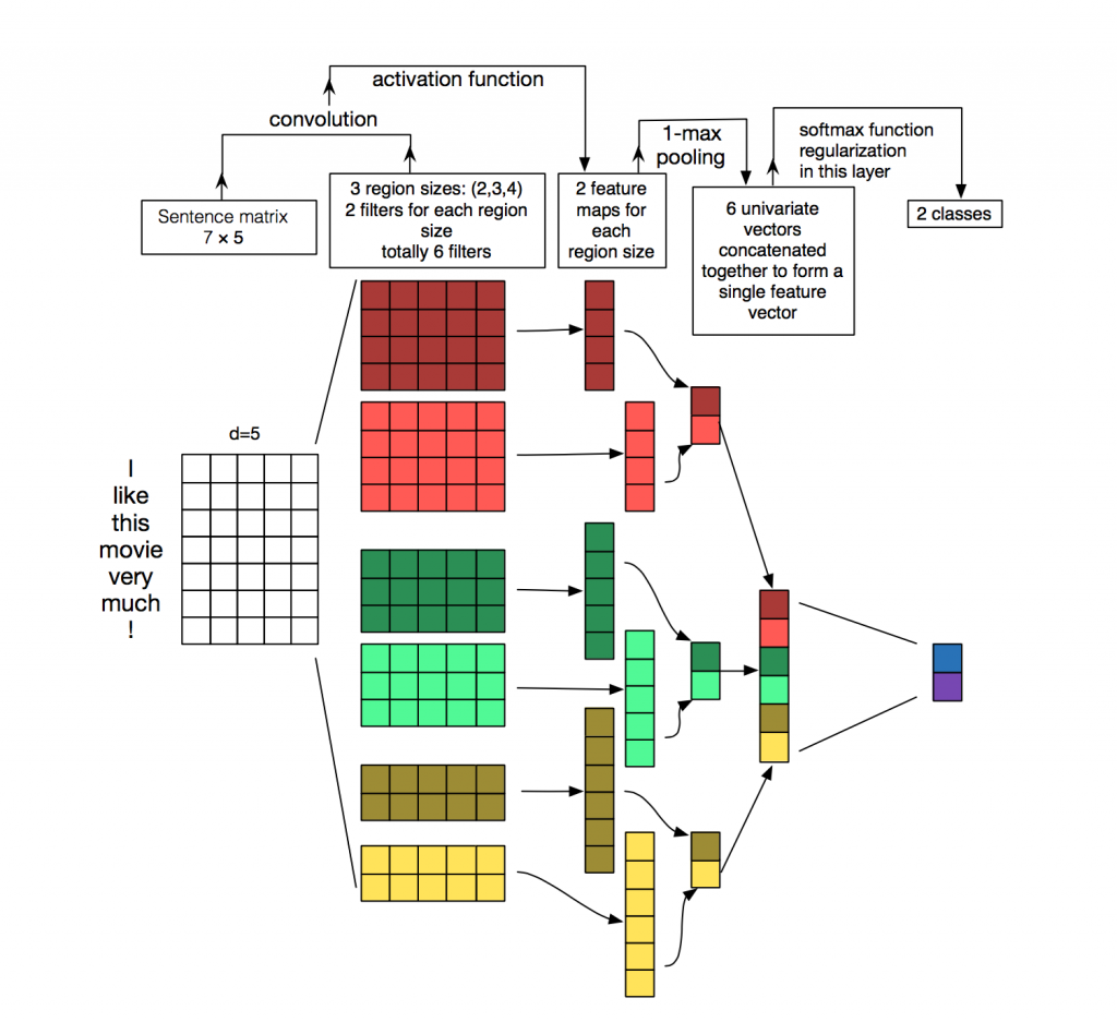
Figure 5: CNN for Natural Language Processing [4]

Multinominal Naive Bayes

The algorithm used to create a benchmark is Multinominal Naive Bayes (MNB). MNB is an approach going one step further that the binomial Bernoulli Naive Bayes (BNB). BNB is a discrete data Naive Bayes classification algorithm, requiring binary input exclusively, meaning it can be only applied to data, consisting of boolean features. In the context of text classification a possible application of BNB would be in case of having data which consists of binary feature vectores (0 & 1), where 0 would mean that a word occurs in a document and 1 would that a word does not occur in a document. On the other hand, MNB’s applicability is not limited to binary data - meaning a MNB can be used when having a feature vector consisting of the count of each word in a document (instead of solely a binary representation of a word’s presence or absence in this document). An example of such vectors can be seen in Figure 6, which represents the so called document term matrix. The matrix contains all the words (or a predefined threshold which only considers the 200,300 etc. most frequent words) found in all documents, which in the current case are tweets and how often a word can be found in each document (tweet), meaning each row of the matrix is a tweet in the context of this project. In the case of BNB such matrix would be binary and filled with 0 and 1 only. To create the matrix, the method “fit_transform” from CountVectorizer is used. It learns the vocabulary from the train set and returns the corresponding document term matrix. Afterwards the test set is transformed to a document term matrix by the function “transform” (also from CountVectorizer). Both matrices are then fed to the MNB Classifier. The algorithm has the parameters “alpha”, “fit_prior” and “class_prior”. “Alpha” is a smoothing parameter, which implies no smoothing if assigned 0 and maximal smoothing if assigned 1. The “fit_prior” determines whether the model should learn class prior possibilities or not. The default setting is TRUE. If set to FALSE, a uniform prior is assumed. Finally, “class_prior” contains the prior probabilities of the classes. If no probabilities are handed, the priors are adjusted according to the data, which is the current case. The accuracy reached with MBN is 75%, which is lower than the accuracy reached by FastText (81.8%) and the CNN (79.8) after hyperparameter optimization [8].

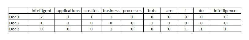
Figure 6: Document Term Matrix [1]

Data preprocessing

Data Cleaning

The first step of the data preprocessing is to clean the gathered pre-labeled tweets [5]. This involves converting all words in the tweets to lower case, unfolding contractions (for example couldn”t to could not), removing special characters, numbers, hashtags, mentions as well as punctuation. Furthermore, the emojis are also removed from the combined dataset. This is done in order to prevent potential overfitting. One part of the entire dataset consists of tweets labeled based on the emojis as already mentioned. Thus, not removing the emojis could lead to good results on the labeled data but poor ones on the unlabeled tweets. Next, each of the tweets is lemmatized. In natural language processing (NLP), lemmatization refers to reducing the different forms of the words in a sentence to the core root (for example the words “walking” and “walked” are transformed to “walk”). Afterward, the stop words are removed from the tweets. Stop words are commonly used words which introduce noise in the data in NLP tasks as they have no informative-value. The library nltk is used in order to retrieve a set of stopwords. It is important to highlight that this set is adjusted by removing the negations from it. The reason for this is that negations like “not” or “no” could have an impact on the correct prediction of the positive and negative sentiment of the tweets. For example several negations in a tweet could serve as an indication for a negative sentiment. Therefore, the reduced set of stop words is used in the cleaning process of the tweets.

Several self-defined functions implement what has been described in the paragraph above. To extract only the text from the tweets and leave HTML characters out, the package BeautifulSoup is used. This package finds application when one needs to pull only text data out of HTML or XML files, using the integrated “get_text” method.
The second issue the cleaning function handles is replacing the “\x92” with a reverse single quote (which is meant to be an apostrophe in texts). It is important explaining briefly why the “\x92” is in the text in a first place. “'” is encoded as “\x92” in CP-1252/Windows-1252 (a single-byte character encoding system). However, “\x92” in CP-1252 encoding is “\x2019” in Unicode Strings encoding, which is a single reverse quote. Since Python 3.0 uses Unicode Strings instead of Bytecode Strings, it does not recognize the encoding and does not show it as “'". Thus, the replacement need to take place manually, as it does via the replace() function, which is inbuilt in Python.
The hashtags, the account name, the URLs and the punctuation in a tweet are removed with the sub() method of the “re” module. This function makes makes replacements of regular expressions. A regular expression is a set of strings that match a criteria. It can also be seen as the opposite of a perfect match to a criteria. The first argument of “re.sub()” is the regular expression, the second one the replacement to be made and the third one the string to be processed (the tweets in this case).
Finally, the cleaning method deals with emojis and contractions. A part of the list of contractions looks as follows:

def load_dict_contractions():

    return {
        "ain't":"is not",
        "amn't":"am not",
        "aren't":"are not",
        "can't":"cannot",
        "'cause":"because",
        "couldn't":"could not",
        "couldn't've":"could not have",
        "could've":"could have",
        "daren't":"dare not",
        "daresn't":"dare not",
        }

This dictionary is then used in the cleaning function in order to replace any abbreviations and slang with the grammatically correct and complete form of an expression. A part of the list of emojis looks as follows:

def load_dict_smileys():

    return {
        ":‑)":"",
        ":-]":"",#"smiley",
        ":-3":"",#"smiley",
        ":->":"",#"smiley",
        "8-)":"",#"smiley",
        ":-}":"",#"smiley",
        ":)":"",#"smiley",
        ":]":"",#"smiley",
        ":3":"",#"smiley",
        ":>":"",#"smiley",
        "8)":"",#"smiley",
        ":}":"",#"smiley",
        ":o)":"",#"smiley",
        }

It serves as a dictionary of actually inexisting (unintentionally wrongly written) emojis. The dictionary is afterwards used in the cleaning function to replace the inexisting emoji with a natural language word (e.g. smiley, sad etc.), which summarizes the emotion the emoji was supposed to express, its actual meaning which is relevant for the sentiment analysis. Last, the function replace() of the library demoji is used to remove all the emojis predefined in the Unicode Consortium’s emoji code repository (needs to be downloaded first by demoji.download_codes()).

def tweet_cleaning_for_sentiment_analysis(tweet):    

   #Escaping HTML characters
   tweet = BeautifulSoup(tweet).get_text()

   #Special case not handled previously: Reverse single quote
   tweet = tweet.replace('\x92',"'")

   #Removal of hastags/account
   tweet = ' '.join(re.sub("(@[A-Za-z0-9]+)|(#[A-Za-z0-9]+)", " ", tweet).split())

   #Removal of address (URL)
   tweet = ' '.join(re.sub("(\w+:\/\/\S+)", " ", tweet).split())

   #Removal of Punctuation
   tweet = ' '.join(re.sub("[\.\,\!\?\:\;\-\=\*\)\(]", " ", tweet).split())

   #CONTRACTIONS source: https://en.wikipedia.org/wiki/Contraction_%28grammar%29
   CONTRACTIONS = load_dict_contractions()
   tweet = tweet.replace("’","'")
   words = tweet.split()
   reformed = [CONTRACTIONS[word] if word in CONTRACTIONS else word for word in words]
   tweet = " ".join(reformed)

   #Deal with emoticons source: https://en.wikipedia.org/wiki/List_of_emoticons
   SMILEY = load_dict_smileys()  
   words = tweet.split()
   reformed = [SMILEY[word] if word in SMILEY else word for word in words]
   tweet = " ".join(reformed)

   #Deal with emojis
   tweet=demoji.replace(tweet,"")
   tweet=remove_emoji(tweet)

   tweet = ' '.join(tweet.split())

   return tweet

Word Embeddings: GloVe and FastText

In NLP tasks machine learning models preprocess textual data with the help of the numerical representation of the words contained in it. In this context, word embeddings are regarded as the dominant approach. They consist of numerical vectors that capture the linguistic meaning of the textual data. In this research two models are used to obtain the word embeddings for the retrieved twitter data. The first one is GloVe that among others provides word embeddings trained on twitter data. The dimension size of the GloVe twitter embeddings is 200. The second model is FastText. It is trained on the cleaned pre-labeled tweets in the unsupervised mode with both CBOW and Skipgram. The dimension of the trained embeddings is also set to 200 in order to ensure comparability of the results. Next, three embedding matrices are generated by using the word vectors from the three models. Each of the tweets in the pre-labeled data is tokenized into single words and the corresponding embedding vector for each word is saved in the embedding matrices. Next the cleaned pre-labeled twitter data is preprocessed according to the requirements of the two machine learning models applied in this research.

Model specific Data Preprocessing

Data Preprocessing CNN

In the embedding layer of the CNN one of the parameters that has to determined in advance is the input length of the data which has to be identical for all tokenized tweets. For this reason the maximal length that each of the tokenized samples can reach is determined by examining the distribution of the length of all tweets. The maximal length is set to 300 as only several tweets in the entire cleaned dataset contain a bigger amount of words than this value. Then the pre-labeled data is padded according to the maximal length in order to ensure that all tokenized tweets have the same length.

Data Preprocessing FastText

FastText does not require the data to be tokenized. For the training of the analytical model developed by Facebook, the labels from the training set are concatenated to the corresponding tweets in a string format with the prefix label. For example, the tweet “I am quite unhappy with some recent developments in politics lately” has the label “0”. The corresponding training record that can be fed to FastText looks in the following way: label 0 I am quite unhappy with some recent developments in politics lately.

Performance Evaluation

Initial Results

Both CNN and FastText are tested with the embedding matrices described in Section 4 in order to examine which word vectors should be used in the next steps. Figure 7 and 8 provide an overview of the initial results. It is important to mention that FastText is also trained without providing any input to the parameter pretrainedVectors. This implies that the embedding matrix is randomly initialized with values between -1/200 and 1/200. Both analytical models achieve the best performance in terms of accuracy with the Twitter pre-trained embeddings from GloVe. Therefore, the GloVe word representations are used in the further analysis of the results.

Figure 7: Initial Results CNN

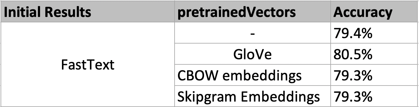
Figure 8: Initial Results FastText

Hyperparameter Tuning using Bayesian Optimization

The hyperparameters of the two models are optimized by using Bayesian Optimization (BO). The library scikit-optimize which is used for the modeling phase applies Gaussian Process (GPs) for the BO. In the context of hyperparameter tuning, GPs are regarded as the surrogate model of the objective function. The later is the evaluation metric according to which the optimal hyperparameters are chosen, for example accuracy, precision, recall etc. The surrogate model learns the mappings between the already tested hyperparameters and the achieved scores by the objective function. The next set of hyperparameter values is chosen according to a selection function, for example the Expected Improvement (EI). The set of configurations that leads to the highest EI is chosen for the next call to the objective function. In this way fewer calls are made to the objective function with hyperparameters that are expected to lead to better results.

Hyperparameter Optimization FastText

Figure 9 contains the five tested hyperparameters of FastText, the corresponding value ranges, the final optimal set of configurations and the highest achieved accuracy. It can be seen that the model developed by Facebook performs best when the feature space of each sentence contains not only words, but also trigrams and character n-grams of a maximal length of 1. Furthermore, the optimal hyperparameters lead to a slight increase in the accuracy of 1.5% compared to the initial results of FastText using the GloVe embeddings.

Figure 9: FastText Hyperparameters

Hyperparameter Optimization CNN

The following function is used to generate the CNN architecture while looping through the different sets of tested configurations.

def CNN_architecture(number_conv_layers,number_filters,pooling_layers,kernel_regularizers_cv,kernel_regularizer_prefinal_dense,
                            units_dense,dp_dense,weight_decay,learning_rate,kernel_size,
                            nb_words, embed_dim,embedding_matrix,max_seq_len):

  model = Sequential()
  # Add the Embedding layer first:
  model.add(Embedding(nb_words, embed_dim,
            weights=[embedding_matrix], input_length=max_seq_len, trainable=False))
  #Make a loop that keeps on adding convolutional layers according to a pre-specified amount.
  for i in range(0,number_conv_layers):
    #Choose between applying L2 Regularization in the convolutional layers or not:
    if kernel_regularizers_cv==True:
      model.add(Conv1D(number_filters,kernel_size, activation='relu',kernel_regularizer=regularizers.l2(weight_decay)))
    else:
      model.add(Conv1D(number_filters,kernel_size,activation='relu'))
    #Make sure that in case maxpooling layers should be added,
    #this is done till the pre-last convolutional layer is reached.
    #For example if 4 convolutional layers have to be added, then 1-3 convolutional layers
    #will be followed by a maxpooling layer, the forth one: not
    last_index_loop=number_conv_layers-1
    if i < last_index_loop:
      if pooling_layers==True:
        model.add(MaxPooling1D(2))

  #Add a global maxpooling layer after the last convolutional layer.    
  model.add(GlobalMaxPooling1D())
  #Choose between applying L2 Regularization in the pre-final dense layer or not:
  if kernel_regularizer_prefinal_dense==True:
    model.add(Dense(units_dense, activation='relu',kernel_regularizer=regularizers.l2(weight_decay)))#, kernel_regularizer=regularizers.l2(weight_decay)))
  else:
    model.add(Dense(units_dense, activation='relu'))

  #Choose between adding a dropout layer after the pre-final dense layer or not:
  if dp_dense==True:
    model.add(Dropout(0.2))

  model.add(Dense(1, activation='sigmoid'))
  #Use Adams for the training process:
  opt=optimizers.Adam(lr=learning_rate)
  model.compile(optimizer=opt,loss='binary_crossentropy', metrics=['accuracy'])

  return model

Figure 10 contains the tested hyperparameters of CNN. It can be seen that the CNN performs best with two convolutional layers. There is an increase of 1.6% in the accuracy compared to the initial performance of the CNN with the GloVe Embeddings.

Figure 10: CNN Hyperparameters

Analysis of the Results on unlabeled Twitter Data

Figures 11 and 12 show several examples of how the tweets are classified (Trump and Booker). For each tweet both the predicted labels and their corresponding probabilities are printed out. The label, which has the higher probability, is considered to be the correct one by the algorithm. The example tweets show best the difference between a positive and negative sentiment. Thus, one must be careful when using sentiment analysis for opinion modeling.

Figure 11: Trump Positive & Negative Sentiment

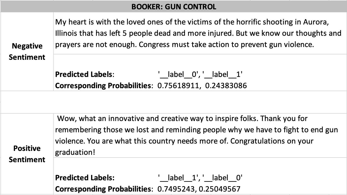
Figure 12: Booker Positive & Negative Sentiment

Figures 13 to 17 show the ratio of positive and negative sentiments for all candidates as classified by FastText in the way described above. As it can be seen all of the candidates have a higher percentage of negative sentiments in their tweets.

Figure 13: Trump Gun Control

Figure 14: Sanders Gun Control

Figure 15: Warren Gun Control

Figure 16: Biden Gun Control

Figure 17: Booker Gun Control

As shown in Figures 11 and 12 a negative sentiment often relates to expressing sadness or disappointment from a violent shooting act or from the current state of the issue. Hence, it is important pointing out that a negative sentiment indeed does not mean that the corresponding candidate is against gun control or pro gun violence. The results from this research show that the negative sentiment strongly relates to a pro gun control setting. In comparison to the negative sentiment, the positive one expresses happiness and satisfaction of an anti gun-violence events. Therefore, the positive sentiment is related to approval of measurements taken into action for ending gun violence.

Conclusion

Since the explored topic is one with a positive conotation (gun control which can also be seen as a part of violence control), it was initially expected that a very high percentage of the tweets would belong to the positive sentiment, because the politicians would “support a positive idea”. However, as the results demonstrate, the majority of the tweets belong to the negative sentiment. However, this does not mean that the candidates do not support gun control (as seen when looking at the content of the tweets). This shows that one cannot blindly draw conclusions simply from the label of a tweet and that a sentiment analysis does not necessarily represent a basis for deriving someone’s opinion on a certain topic, meaning a positive/negative sentiment is not necessarily a reflection of a positive/negative opinion or setting.

References

[1] Bishop, D. (2017). Text Analytics – Document Term Matrix. http://www.darrinbishop.com/blog/2017/10/text-analytics-document-term-matrix/. Accessed on: 07.01.2020.

[2] Böhm, T. (2018). The General Ideas of Word Embeddings. https://towardsdatascience.com/the-three-main-branches-of-word-embeddings-7b90fa36dfb9. Accessed on: 12.12.2019.

[3] Bressler, D. (2018). Building a convolutional neural network for natural language processing. https://towardsdatascience.com/how-to-build-a-gated-convolutional-neural-network-gcnn-for-natural-language-processing-nlp-5ba3ee730bfb. Accessed on: 05.11.2019.

[4] BRITZ, D. (2015). Understanding Convolutional Neural Networks for NLP. http://www.wildml.com/2015/11/understanding-convolutional-neural-networks-for-nlp/. Accessed on: 10.12.2019.

[5] Doshi, S. (2019). Twitter Sentiment Analysis using fastText. https://towardsdatascience.com/twitter-sentiment-analysis-using-fasttext-9ccd04465597. Accessed on: 13.11.2019.

[6] KULSHRESTHA, R. (2019). NLP 101: Word2Vec — Skip-gram and CBOW. https://towardsdatascience.com/nlp-101-word2vec-skip-gram-and-cbow-93512ee24314. Accessed on: 15.01.2020.

[7] Mestre, M. (2018). FastText: stepping through the code. https://medium.com/@mariamestre/fasttext-stepping-through-the-code-259996d6ebc4. Accessed on: 09.01.2020.

[8] Raschka, S. (2014). Naive Bayes and Text Classification – Introduction and Theory. http://sebastianraschka.com/Articles/2014_naive_bayes_1.html. Accessed on: 15.12.2019.

[9] Subedi, N. (2018). FastText: Under the Hood. https://towardsdatascience.com/fasttext-under-the-hood-11efc57b2b3. Accessed on: 13.12.2019.