By Seminar Information Systems (WS 19/20) | February 6, 2020
State of the Art Summarisation Techniques
Generating Headlines as Short Summaries of Text
Information Systems Seminar 19/20
Anna Franziska Bothe
Alex Truesdale
Lukas Kolbe
Abstract
This project combines two NLP use cases: generation of text summaries (in the form of short news headlines) and classification of a given article as containing or not containing political / economic uncertainty. The two approaches are joined by generating a set of new headlines alternative to the original headlines for each article in the given article set. The two headlines are then compared in their performance as inputs in a classification model. While the high-level exercise here is to examine the information value of news headlines in this classification task, the bulk of this blog post examines more closely the inner workings of sequence-to-sequence text modeling in the context of summary generation. The seq2seq model produced in this post, even in a relatively basic form, successfully generates coherent headlines for many of the articles provided. While not every single generated headline is of high quality, there are numerous examples where the headline fits the contents of the article quite well. In general, longer inputs to the model produce better output than short inputs, even though they undergo more thorough text cleaning in pre-preparation (i.e. removal of overly common or rare words).
For the classification task, in comparing the performance of a simple classifier neural network across different input data combinations, the input of article text plus the original headline performs best. Using article text without any headlines gives the second best score and provides better classification results than the input of article text plus a generated headline. This demonstrates that the summarisation model in its current state has potential for improvement. As an academic pursuit & practical application, however, the successful application of several NLP principles in producing a working text generation model is an encouraging achievement with promising potential.
Introduction
The Internet and computer technology make possible low-barrier access to immeasurable amounts of information. While the opportunities here are great and wide-reaching, so too are the challenges, namely the limitations of the human brain to process such large amounts of information in a useful and efficient way.
Additionally, as access to information has grown, so too has the line between factual and fake information begun to blur. Due to the extreme amount of information generated and disseminated on a daily basis, it has become increasingly difficult to identify useful, interesting, and legitimate content. Furthermore, revenue for online publications is very often tied to the amount of page visitors they receive, thereby incentivising article headlines that grab reader attention rather than those that focus solely on conveying information.
In this context, there are many application possibilites for Natural Language Processing (NLP) models to perform tasks that address these challenges: they can, for example (pre-) qualify content through classification, translate text, or, as is the primary focus of this post, serve automatically generated summaries:
-
extractive summarisation is a more basic solution that extracts the most important words or sentences without “writing” any new content on its own
-
more sophisticated and promising, abstractive summarisation models learn to understand language in its nuance (syntax & context) and generate summarizations using “its own words”.
This blog post will first provide an overview of contemporary summarisation techniques in the context of abstractive summarisation. After introducing the methodology, a detailed walkthrough of construction of a sequence-to-sequence model is given. This model will generate short summaries (headlines) of up to 20 words for news articles.
The quality of the generated headlines will be evaluated via common text-generation performance metrics ROUGE and BLEU as well as looking at the performance of these headlines in the final classification task. The quality of these measurements is then compared to that of the actual headlines written by journalists (original data). Does a trained model pick up the context of a medium-to-long article and condense it into a headline that makes sense? That encapsulates central ideas / themes of an article? Can a generated headline contain less bias than one written by a human? These are the driving questions of this analysis.
Outline
- Model Architecture
- Sequence2Sequence
- Encoder-Decoder
- Attention
- Dataset
- Data Cleaning
- Training Strategy
- Model Summary & Code Implementation
- Sequence2Sequence
- Attention
- Encoder-Decoder with Attention
- Inference Model & Text Generation
- Model Results & Performance
- ROUGE
- BLEU
- Evaluation Results
- Classification Model
- Outlook: Potential Enhancements
- Increase Efficiency: Beam Search
- Increase Accuracy: Pointer-Generator Network
- Penalize Repetition: Coverage
- Closing Comment
Disclaimer
For brevity and reading comprehension, only essential code is contained in this blog post. For the full code please refer to the project’s GitHub repository.
Model Architecture
Sequence2Sequence
The concept of sequence-to-sequence (seq2seq) modeling was first introduced by Sutskever et al. in 2014. [4] In its basic functionality, a Seq2Seq model takes a sequence of objects (words, letters, time series, etc) and outputs another sequence of objects. The ‘black box’ in between is a complex structure of numerous Recurrent Neural Networks (RNNs) that first transfers an input string (in the case of seq2seq for text transformation) of varying length into a fixed length vector representation, which is then used to generate an output string.
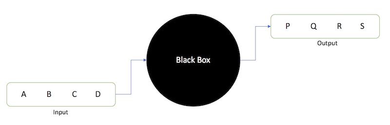
Figure 1: Basic Seq2Seq Model – Image Source: https://towardsdatascience.com/day-1-2-attention-seq2seq-models-65df3f49e263
There are several flavours of seq2seq models, and, depending on the type of problem, the right sub type has to be selected. In this case of text summarisation, the most appropriate application is a ‘many to many’ model where both the input and output consist of several (many) words.
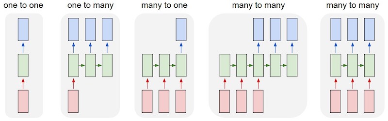
Figure 2:Different Seq2Seq Model Types – Image Source: http://karpathy.github.io/2015/05/21/rnn-effectiveness
Examples:
- One to one: image classification
- One to many: image captioning
- Many to one: text classification
- Many to many: text translation, text summarisation
Encoder-Decoder
Now, the contents of the ‘black box’ in the diagram above can be examined. Sequence to sequence models rely on what is called an encoder-decoder architecture – a combination of layered RNNs that are arranged in way that allows them to perform the tasks of encoding a word sequence and then passing that encoded sequence to a decoder network to produce an output [15][16]. The input sequence is first tokenised (transformed from a collection of words into a collection of integers that represent each word) and then fed word-for-word into the encoder. The encoder transforms the sequence into a new, abstracted state, which then, after being passed to the decoder, becomes the basis of producing an output sequence (e.g. a translated version of the same text, or, in this case a summarised version of the same text).
What does the Encoder do?
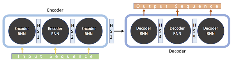
Figure 3: Encoder Decoder Model Scheme – Image Source: https://towardsdatascience.com/day-1-2-attention-seq2seq-models-65df3f49e263
The encoder reads the entire input sequence word by word, producing a sequence of encoder hidden states. At each time step, a new token is read and the hidden state is updated with the new information. Upon reaching the end of the input sequence, the encoder puts out a fixed length representation of the input, regardless of input length, which is called the encoder vector. The encoder vector is the final hidden state that is used to initialize the decoder.
What does the Decoder do?
In contrast to the encoder, which takes in input data and reflects in a final, abstracted state, the decoder is trained to output a new, fixed-length sequence (word-for-word) given the previous word for each time step. It is initialized by receiving the encoder vector as its first hidden state, as well as a “start”-token, indicating the start point of the output sequence. The true output sequence is unknown to decoder while decoding the input sequence, it only knows the last encoder hidden state and the previous input (the “start” token or the next token from the input sequence), which it receives at each time step. The decoder has the ability to freely generate words from the vocabulary.
Limitations with Encoder-Decoder Architecture:
While the LSTM or GRU units in the encoder-decoder architecture are well suited for contextual analysis of inputs, they begin to struggle with this task as inputs grow longer. With long input sequences, the final state vector that is output by the encoder may lose important contextual information from earlier points in the sequence [13][14]. Through every iteration of the encoder RNN, hidden states are updated by new information, slowly moving away from early inputs. The core problem here is that the entire context of the long input text is condensed into one single state vector.
Intuition: imagine the challenge of reading a whole text once, then writing a summary from memory – it becomes difficult to remember the early details of the original text.
Attention
One solution to the above-mentioned issue is called attention. Attention serves to assist the encoder-decoder model in specifically focusing on certain, relevant sections / words in the input text when predicting the next output token. This helps to mitigate the issue of lost context from earlier chunks of an input sequence. With attention, instead of a one-shot context vector based on the last (hidden) state of the encoder, the context vector is constructed using ALL hidden states of the encoder.
Intuition: imagine the challenge reading a whole text once whilst writing down keywords and then writing a summary – with these notes, it becomes much easier to condense the key ideas from the entirety of the original text.
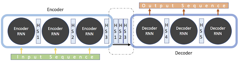
Figure 4: Encoder Decoder Model with Attention – Image Source: https://towardsdatascience.com/day-1-2-attention-seq2seq-models-65df3f49e263
When combining the hidden states into the final encoder output (decoder input), each vector (state) gets its own random weight. These weights are re-calculated by the alignment model, another Neural Network trained parallel to the decoder which checks how well the last decoder output fits to the different states passed over from the encoder. Depending on the respective fit scores, the alignment model weights are optimized via back propagation. Through this dynamic weighting, the importance of the different hidden states varies across input-output instances, allowing the model to pay more attention (weight / importance) to different encoder states based on the input. [Source: https://towardsdatascience.com/attn-illustrated-attention-5ec4ad276ee3]

Figure 5: Attention Principle – Image Source: https://github.com/google/seq2seq
Attention in Detail
In this blog’s model, Additive/“Bahdanau” Attention [3] is used. This method works as follows:
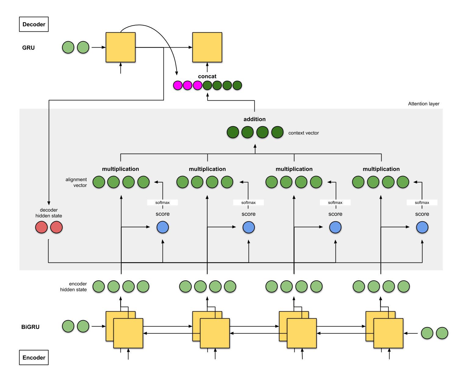
Figure 6: Detailed Diagram of Additive Attention – Image Source: https://towardsdatascience.com/attn-illustrated-attention-5ec4ad276ee3
- The encoder reads input text (in both directions in the case of a bi-directional GRU / LSTM) and produces hidden states for each time step
- The combined encoder state is the first input to the decoder
- The decoder puts out the first decoder hidden state
- A score (scalar) is obtained by an alignment model, also called score function (blue)
- In this blog’s model, this is an addition / concatenation of the decoder and encoder hidden states (i.e. tensors)*
- The final scores are then obtained by application of a softmax layer
- Each encoder hidden state is then multiplied by its scores/weights
- All weighted encoder hidden states are then added together to form the context vector (dark green)
- The input to the next decoder step is the concatenation between the generated word from the previous decoder time step (pink) and context vector from the current time step.
*many other scoring functions are possible
Dataset
The data in this application is a collection of 376.017 news articles from various US newspapers. This collection includes news articles and headlines, date of publication, source publication, and a binary classification score denoting presence of political / economic uncertainty in the article. This classification is done via checking for the presence of certain words in the article text. In preparing the data for modeling, cleaning is performed on headlines and texts needed for supervised training.
Data Cleaning
The cleaning process consists of a combination of standard processes and custom, domain-specific cleaning steps. Headlines and body text are processed separately, as they each contain unique sets of impurities. First, duplicate rows are removed, as are any articles of newspapers with less than 100 appearances (these are overwhelmingly noisy data points). Rows with NULL values in either headline or body text are also removed.
The remaining data comprises ~300.000 rows (articles) from 10 news sources:
- The Washington Post
- Pittsburgh Post-Gazette (Pennsylvania)
- The Atlanta Journal-Constitution
- St. Louis Post-Dispatch (Missouri)
- USA Today
- Star Tribune (Minneapolis, MN)
- The Philadelphia Inquirer (Pennsylvania)
- St. Petersburg Times / Tampa Bay Times (Florida)
- The Orange County Register (California)
- The New York Post
Upon closer inspection, a significant number of very-near-duplicates remain in the data set, hallmarked by having the same article text save an extra space or a deviation of 2 to 3 words. To identify and remove these duplicates, a more sophisticated function based on text content is employed. It is important to do so, as having only unique rows in training produces the best conditions for reducing any learned bias in the final model due to doubling or tripling an article-to-headline pair.
This function identifies any duplicate headlines and then examines their respective articles for text similarity using TF-IDF scores. If two articles share a headline and are more than 90% similar in their word composition, they are deemed duplicates and one of them is thrown out. In total, this process identifies and removes ~5.000 additional duplicates (function and example output from cleaning handler below).
Specific publications also contain their own nuances in terms of recurring phrases in article headlines. For this, further cleaning steps tailored to each paper are needed. Full code for these cleaner functions can be found in the project notebook, but an example would be explicit indicators that an article is part of a set or series of publications like ‘SUNDAY CONVERSATION’ or content disclaimers such as ‘POLITICAL’. Source-specific cleaner functions are written by manually examining these commonly occurring n-grams (phrases) and removing them. This prevents the text generation model from learning unimportant, repeating phrases that don’t reliably carry information. Furthermore, obituaries (Nachrufe) posted in the Pittsburgh Post-Gazette are removed, as they present challenges in their syntax idiosyncrasies (a lot of numbers and punctuation) and do not generalise well (are not found anywhere else in the data).
Following these custom data cleaning solutions, standard and well-established procedures are applied:
- Stop- and short word removal
- Case conversion (all lowercase)
- Contraction conversion (manual)
- Remove of punctuation
- Remove of HTML code and URLs
- Conversion of special characters into their verbal representation (e.g. ‘@’ to ‘at’)
- Remove (‘s)
Lastly, rare words and exceedingly common words are removed from both headlines and body text based on word count with thresholds set independently for body text and headlines. This reduces the number of words in the model vocabulary, reducing computation time and complexity, while increasing the chance that the model will be able learn each word’s context. With the inclusion of very rare words, the model might have trouble understanding their meaning, not having enough word occurrences to observe. In source papers, an article vocabulary size of 50.000 is recommended as a suitable intersection between maintaining vocabulary density and sufficiently trimming uncommon words. In this case, that results in a removal of 90% of unique tokens (or ‘words’). The threshold for headlines was chosen as a more conservative application of similar logic, as the headline is the target in the seq2seq model – rather than removing 90% of the headline vocabulary, 60% is removed.
The measures described above result in the following word distributions.
|
Word occurrences in Articles Total words: 508.657 Less than 60 occurrences: 558.693 Remaining words: 55.126 Removing 90\% of words |
Word
occurrences in Headlines Total words: 59.841 Less than 8 occurrences: 37.691 Remaining words: 22.150 Removing 60\% of words |
||
| said | 1.647.581 | new | 15.097 |
| year | 572.948 | tax | 7.708 |
| new | 556.554 | economy | 7.603 |
| percent | 525.136 | obama | 7.258 |
| people | 436.461 | says | 7.035 |
| years | 420.477 | state | 6.695 |
| state | 408.316 | plan | 6.353 |
| million | 336.585 | jobs | 6.043 |
| economic | 332.319 | city | 5.995 |
| time | 330.871 | big | 5.437 |
| president | 323.103 | economic | 5.056 |
As final preparation of input texts for their use in modeling, standardised article and headline lengths must be determined. This is because neural networks require a fixed-length input sequence. In the figure below, the distributions of article lengths (frame 1) and that of headlines (frame 3) are plotted to help in selecting these standard values. Frame 2 shows the distribution of article length for trimmed articles, which will be explained in the next section.
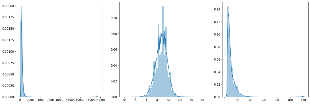
Figure 7: Word length distributions for articles and headlines
The standard article length value of 550 is selected, as 83% of the articles fall below this number. The idea here is to be conservative in minimising the amount of truncated articles that go on to model training while at the same time restricting article length as much as possible to avoid working with inputs that are too large. In selecting standard headline length, all rows with a length greater than the standard values are removed from the set. For this reason, the value is set high (at 20) to ensure that the maximum number of data points from the incoming data are retained (93%). Rows with headlines exceeding this value must be removed because each headline must be fitted with start and end tokens at its beginning and end for both model training and, ultimately, text generation.
Training Strategy
An additional step is the examination of the hypothesis that much of an article’s content is present simply in its first x-words and that the remaining text is just further exposition of the already-outlined topic(s). To test this idea, the data is forked at this point to include the aforementioned articles of length 550, as well as a trimmed set where the articles are truncated beyond a maximum length of 80 words (tokens). This approach is inspired by findings in the literature where seq2seq models in similar tasks struggled to beat a baseline model that generated summaries simply by extracting the first three sentences [2].
In the case of the longer articles, extensive removal of rare words is carried out (as explained above). For the trimmed articles, a less strict removal of rare words (reducing the threshold that classifies a word as ‘rare’) is applied. The idea here is that a shorter but more complete excerpt of the input text (that in itself effectively captures the context of the article) might be well suited for training the model from which headlines are generated. I.e. if the headline matches the first 80 tokens well, it will likely also be a suitable headline for the whole text. The following two data sets are carried through as inputs for seq2seq models, which are then measured against each other based on validation loss during model training.
1) “Generous input, thorough trimming”
Articles:
- larger inputs (550 tokens)
- thorough removal of rare words (fewer than 60 occurrences), leaving 10%/50k words
Headlines:
- 20 tokens max.
- remove words with fewer than 8 occurrences, leaving 35%/22k words
2) “Truncated inputs, little trimming”
Articles:
- small inputs (50 tokens)
- only removing words with fewer than 10 occurrences: 25%/40k words
Headlines as above
Model Summary & Code Implementation
![Figure 8: Encoder-Decoder Net with Attention – Image Source: [2] Abigail See 2017](/blog/img/seminar/is1920_group9/architecture_1.png)
Figure 8: Encoder-Decoder Net with Attention – Image Source: [2] Abigail See 2017
Sequence2Sequence Model
The model architecture employed in this project is inspired by [2] Abigail See et al. (2017) and her similar text summarisation task. Also, Aravind Pai’s blog post ‘Comprehensive Guide to Text Summarization using Deep Learning in Python’ [12] was used as a guideline for some parts of the implementation. The model in this blog differs in that it uses two bi-directional Gated Recurrent Units (GRUs) instead of one bi-directional Long-Short-Term-Memory (LSTM) Network. GRUs are chosen for their equal performance [5] while providing superior computational efficiency in training. Additionally, bi-directional GRUs are the RNN of choice in experiments by Bahdanau et al. in their introduction of their attention mechanism [3]. Lastly, pre-trained word embeddings are employed instead of training embeddings on local data alongside model training. These pre-trained embeddings come from the GPT-2 project. The GPT-2 embeddings are chosen, as they are likely the most robust and generalisable available. These embeddings are trained on 40GB of Internet text and are part of the most advanced, state-of-the-art transformer model currently in production. Finally, the model is implemented in python, using Tensorflow / Keras.
The encoder is set up using two bi-directional GRUs with a latent dimension of 256. The first GRU passes its output to the second, which then processes all previous hidden states and produces an output layer containing the second GRU’s step wise hidden states and a final hidden state. Since the GRUs are bi-directional, there is both a forward and a backward state which are combined (concatenated) as the encoder state.
Once the input is processed, the decoder GRU begins outputting a sequence that is the summary sequence. At each step, it receives the encoder hidden states and the previous decoder output as its input, updates the decoder hidden states, and selects a new token as this step’s decoder output. The decoder is set up as a single, mono-directional GRU (it produces text only in the forward direction). It receives unique embeddings of the headlines, as they have a different vocabulary than the articles, and is initialized with the combined encoder state (final encoder hidden layer).
Attention
![Figure 9: Encoder-Decoder Net with Attention – Image Source: [2] Abigail See 2017](/blog/img/seminar/is1920_group9/architecture_2.png)
Figure 9: Encoder-Decoder Net with Attention – Image Source: [2] Abigail See 2017
The encoder and decoder outputs (hidden states) are fed into the attention layer. The AttentionLayer() function does two things (simplified as ‘attention distribution’ in the figure above): It checks the alignment of the current decoder hidden state with each encoder hidden state, using concatenation as a scoring function, and then runs the obtained attention scores through a softmax layer. Using the attention distribution from the decoder, a weighted sum of the encoder hidden states is produced. This is called the context vector. This vector can be regarded as “what has been read from the source text” at this step of the decoder.
In the final step, the context vector and the decoder hidden state are concatenated and fed through a softmax-activated dense layer to receive the vocabulary distribution, attaching probabilities to each word in the vocabulary. The word with the highest probability is then chosen as the next output.
The code for the AttentionLayer() was sourced from Thushan Ganegedara
- Blog post: https://github.com/thushv89/attention_keras
- github: https://towardsdatascience.com/light-on-math-ml-attention-with-keras-dc8dbc1fad3
Encoder-Decoder Model with Attention
The specifications above result in the following model and training results:
Training with Long Articles
Training with Short Articles
As seen in the two above code blocks, while training was considerably quicker with the shorter inputs, the validation loss is lower for the data subset with the longer articles. Based on this metric, the longer articles are selected as inputs for the language (seq2seq) and classifier models from here forward since we want to maximize performance.
Inference Model & Text Generation
For the inference phase, the decoder is set up slightly differently than before. In order to obtain headline predictions for test data, the following steps are necessary:
- Encode the input sequence into an encoder vector
- Start with a target sequence of size 1 (just the start-of-sequence token)
- Feed the state vectors and 1-token target sequence to the decoder to produce predictions for the next token
- Sample the next token from the vocabulary using these predictions (greedy search / argmax)
- Append the sampled token to the target sequence
- Repeat until the end-of-sequence token is generated or the maximum headline length is reached
Below are 10 output examples drawn from the model output data frame:
| Article (first 20 tokens) | Original headline | Generated headline |
|---|---|---|
| sweltering afternoon july affordable housing advocates religious leaders new jerseys influential officials arrived mount laurel celebration years making legislature gov corzine | affordable housing advocates now calling for delays in nj | affordable housing bill is a step in affordable housing |
| bankruptcy largely matter semantics know going going bankruptcy outside bankruptcy system benefit courts maryann keller written auto industry decades end day | detroit prepare for big changes automakers future paved with pain | detroit automakers face tough road to bankruptcy |
| confessed pension wars conjure watchdog nerdy high school chemistry teacher terrific crush chant changes half life aloud unison talking radioactivity course | pension promises can be altered lawyer says | pension reform should be a better way |
| chilean dictator gen augusto pinochet target numerous human rights prosecutions suffered heart attack early yesterday morning hospitalized stable condition controversial year | pinochet hospitalized after heart attack the former chilean dictator surgeries he is been the target of human rights prosecutions | former fed official gets a second term |
| minimum wage argue job killer raises costs employers dramatic minimum wage increase solution relieve poverty karen bremer executive director georgia restaurant | recession sharpens ga wage war | low wage workers are not working |
| black gowns square caps wide smiles seniors graduated month bridgewater state college massachusetts appeared perfect slice america lot graduates women men | more women graduate why | where is the college of the american dream |
| today mothers day days miss calendar good son daughter hectic weeks noteworthy moments slipped past finished national awareness day national postal | sorry moms no grand proclamation for you | our opinion letters readers respond to the editor for march |
| great shellacking throw democratic congressional staffers jobs send thousands gleeful republican staffer wannabes overdrive resumes hill fill vacancies envelope look numbers | all the unemployed democrats will the soup kitchens have enough | for the gop job a chance to be a good thing |
| years ago according april edition granite city press record morning remained unemployed relief fund thursday mark end aid granite citys destitute | this week in granite city area history | st louis county gets million in second quarter |
Model Results & Performance
To measure the quality of the generated headlines, two popular evaluation metrics are applied: ROUGE & BLEU. With human evaluation being costly and slow, both of these metrics are designed to efficiently evaluate computer-generated texts and compare the similarity of the generated summary to the reference summary, each method scoring similarity between 0 and 1. The closer the score is to 0, the less similar the summaries are. A score of 1 represents a perfect match between summaries. [8][10]
For this application, evaluation of unigrams is most reasonable and produces the most reliable results; it is less likely to have matching n-grams with n $>$ 1 plus correct word order in very short summaries (in contrast to long summaries). For the following, all concepts and formulas will be explained in the context of unigrams.
Note that ROUGE and BLEU are introduced and applied here, as they are classic evaluation tools for measurement of text model efficacy. They do, however, have some limitations in the context of this blog post’s application (and abstractive summarisation in general). Namely, the two metrics evaluate summaries based on identical word content, and, as such, miss nuances in context-based similarity (i.e. a model producing qualitatively valuable synonyms). Measuring the above seq2seq model’s output with ROUGE and BLEU has some validity but also noteworthy limitations that ideally require some sort of context-based metric for more granular evaluation – something that is not yet available / widely agreed upon in academia or industry.
ROUGE
ROUGE (Recall-Oriented Understudy Gisting Evaluation) is a recall-based evaluation metric. Recall measures how much of the reference summary is captured within the generated summary:
\begin{equation} \frac{\mathrm{Number \ of \ overlapping \ words}}{\mathrm{Total \ number \ of \ words \ in \ reference \ summary}} \end{equation}
Numerous variations of ROUGE exist. Below is a brief summary of the most relevant and common varieties, which are used for text summarisation. As mentioned, the focus will lie on unigram ROUGE evaluation (ROUGE-1) when evaluating results of the summarisation model above.
According to Lin (2004), the methods ROUGE-1, ROUGE-L, ROUGE-W, ROUGE-SU4 and ROUGE-SU9 perform the best on very short summaries such as headlines (average summary about 10 words):
- ROUGE-N: measures the n-grams (such as unigrams = ROUGE-1) overlap of words
- ROUGE-S: measures the skip-bigram co-occurrence, which means that every combination of two words in a sentence are counted; the maximum distance between those two words can be set with the parameter d (d = 0 is equal to ROUGE-2)
- ROUGE-SU4: counts unigrams and skip-bigrams with a maximum distance of 4
- ROUGE-SU9: counts unigrams and skip-bigrams with a maximum distance of 9
- ROUGE-L: measures the “longest common subsequence” (LCS) of words due to the assumption that the longer the matching sequence, the closer the summaries
- ROUGE-W: weights the LCS by counting and comparing the consecutive matches of words; long consectives indicate more similarity between reference and generated sentence
All measures with n-grams with n $>$ 1 are sensitive to word order.
Very short summaries are penalized by dividing the number of overlapping words by the total number of words in the reference summary (see ROUGE-1$_{recall}$ score).
| ID | Reference summary | Generated summary | ROUGE-1recall |
|---|---|---|---|
| A | the grey mouse eats a piece of apple in the house | the mouse eats | 0.27 |
| B | the mouse eats | the grey mouse eats a piece of apple in the house | 1 |
Recall does not penalize very short summaries, though. In case of ID B, the ROUGE-1$_{recall}$ score results in a perfect match which means that the reference and generated summaries are identical. However, by having a look at the example ID B, this is obviously not the case. Therefore, it is always necessary to consider a second metric: precision, which is computed as follows:
\begin{equation} \frac{\mathrm{Number \ of \ overlapping \ words}}{\mathrm{Total \ number \ of \ words \ in \ generated \ summary}} \end{equation}
Precision captures the extent to which the content of the generated summary is actually needed. The precision and recall scores are combined by the F$_{1}$-score which is the harmonic mean of both results. [8][9]
| ID | Reference summary | Generated summary | ROUGE-1recall | ROUGE-1precision | F1-score |
|---|---|---|---|---|---|
| A | the grey mouse eats a piece of apple in the house | the mouse eats | 0.27 | 1 | 0.43 |
| B | the mouse eats | the grey mouse eats a piece of apple in the house | 1 | 0.27 | 0.43 |
If the length of the reference summary is not penalized, this results in a perfect match (see precision result of ID A) because all words of the generated summary occur in the reference summary. In this case, the precision score receives too much weight. For this reason, in the evaluation of the above model’s generated headlines, the F$_{1}$-score of ROUGE-1 is used.
BLEU
BLEU (Bilingual Evaluation Understudy) is a precision-based evaluation metric. It was originally developed for machine translation evaluation. The precision score is computed as presented in the introduction to ROUGE. The number of overlapping words is divided by the total number of words of the generated (not reference, like in the case of ROUGE recall) summary. Analogous to ROUGE, the BLEU metric counts matching unigrams of the generated summary in comparison to the reference summary. The specific position of the words in each summary is not important.
A drawback of precision-based evaluation metrics is the tendency to overvalue repeating words in the generated summary, which leads to a high precision score for what may actually be a summary of low qualitative value.
As an example, consider the reference summary of the ROUGE score above (with a new generated summary):
Reference summary: the grey mouse eats a piece of apple in the house
Generated summary: the the the the the the the the
Sometimes, summarisation models tend to repeated themselves (see coverage in the potential enhancements section). Even though the generated summary is very low quality, the precision score here would be 1 ($\frac{8}{8}$ - 8 matching words divided by the 8-word generated summary), which indicates a perfect summary.
In order to prevent this from happening and to avoid giving too much weight to repeated words, BLEU introduces a modified unigram precision score. After a word of the reference summary is matched once, the word is exhausted and cannot be matched or counted again.
The implementation of this approach is performed via the following steps:
- The maximum number of times a specific words occurs in the reference summary is counted
- The words of the generated summary are only matched as often as the maximal count of each word from 1. (if there is more than one reference summary, the maximum count is the maximum number of times it occurs in a single one of them)
- The number of eligible, matched words of the generated summary is divided by the total number of words in the generated summary
Consequently, the modified precision score of the example presented above is only 0.5 ($\frac{2}{4}$). The target of modified unigram precision, then, is the improvement of the accuracy of the model evaluation.
An additional challenge occurs if the length of the generated summary deviates substantially from the length of the reference. Very long summaries are captured and penalized by precision. Unfortunately, very short ones are not.
Reference summary: the grey mouse eats a piece of apple in the house
Generated summary: the apple
The precision score of the generated summary is 1 ($\frac{2}{2}$), again an indication of a perfect summary, even though it is a visibly bad one. The solution here is a function that works similarly to recall (presented in the ROUGE section above).
Since BLEU was originally constructed for the evaluation of translated sentences in comparison to multiple reference translations of different word lengths, the metric of recall in its original form could not be implemented. Therefore, a brevity penalty factor has been introduced, which looks for the reference with the most similar length:
\begin{equation}
BP =
\begin{cases}
1 & \text{if $c > \ r$} \\\
e^{1-\frac{r}{c}} & \text{if $c \leq \ r$}
\end{cases}
\end{equation}
Let c be the candidate (= generated summary) and r the reference. A brevity factor length of 1 (exp(0)) indicates that the reference and generated sentence have the same length.
Finally, the BLEU metric score is computed as follows
\begin{equation} BLEU = BP * exp(\sum_{n=1}^{N}w_{n}log \ p_{n}) \end{equation}
With p being the precision score. [10]
In this project’s analysis, only one reference is available, making the weights unnecessary. In this case, the BLEU score is calculated simply with
\begin{equation} BLEU = BP * exp(log \ p) \end{equation}
Evaluation Results
The ROUGE and BLEU evaluation output as well as headline results with the given scores are shown and discussed below:
| ROUGE-1 | BLEU | |
|---|---|---|
| Min. / Max. | 0/1 | 0/1 |
| Mean | 0.10912 | 0.09002 |
| Median | 0.09091 | 0.05936 |
Reminder: for both methods, the evaluation scores are based on unigrams. In average the mean of ROUGE scores is somewhat higher than that of BLEU scores. In contrast, the median is 0.03155 lower and thereby deviates from the mean by 0.84084. This indicates that BLEU has some outlier scores. Additionally, both evaluation metrics show a right-skewed distribution and evaluate some summaries as fully identically (1) and completely different (0).
Below are some selected results of the text summarisation task. In general, it can be observed that the ROUGE score is mostly greater or equal to the BLEU score which is the result of a less severe evaluation of the ROUGE metric. Since ROUGE divides the matched words by the total number of words of the original summary, it sometimes has a lower evaluation score than BLEU if the generated summary is shorter than the original.
| ID | Original | Generated | Score ROUGE | Score BLEU |
|---|---|---|---|---|
| 1 | state representative district democrat | state representative district democrat | 1 | 1 |
| 2 | general mills to cut more jobs | general mills to cut jobs | 0.8333333 | 0.8187308 |
| 3 | at and t to purchase t mobile | gm and t to buy t mobile | 0.6666667 | 0.7142857 |
| 4 | your views letters to the editor feb | letters to the editor may | 0.5714286 | 0.5362560 |
| 5 | romney to stress foreign policy | foreign policy foreign policy | 0.40000000 | 0.3894004 |
| 6 | the iraq war will cost us trillion and much more | myths about iraq war | 0.2000000 | 0.1115651 |
| 7 | turning up the heat on climate issue years ago a degree day illustrated scientists warning | climate change is a hot issue | 0.2000000 | 0.1115651 |
| 8 | editorial rio olympics tainted by dark clouds darker waters | rio rio rio and the rio of the rio | 0.1111111 | 0.1111111 |
| 9 | clean energy is inevitable | letters to the editor letters to the editor | 0 | 0 |
| 10 | existing plan for mercury pollution should work well | clean air is a good thing | 0 | 0 |
| 11 | joblessness worse here than year ago | unemployment in region is percent in the month | 0 | 0 |
The model produces summaries that are nearly identical to the original summary (IDs 1 & 2), while also producing some that are nonsensical (ID 9). However, the model also produces good summaries that are not evaluated as such because the evaluation metrics search for equal words and words of semantic similarity. Take, for example, the words joblessness and unemployment (ID 11). Furthermore, sometimes the content is very similar even though the sentence structure (and length) deviates quite a bit (ID 7 & 10). Especially interesting from a headline research perspective are the plausible shifts in headline content such as in example ID 6.
In the beginning of this blog, the idea was introduced that headlines might be sensational in nature for the purpose of drawing attention, while not providing actual information, necessarily. The model produced in this case generates its predictions based on article content (though, worth noting, evaluated using the original headlines). Ideally, this means that the model was sufficiently trained to be informative rather than sensational. Take again ID 6 as an example: the original headline of is “The Iraq war will cost us trillion and much more”. The model in this post model summed up the article as “Myths about Iraq war”. In this case, manual examination of the article content is required to evaluate whether this is an exceptional summary or one that fails to capture the content of the related news story.
Note as well the following two cases in the results table above: some summaries contain falsely exchanged names or single letters (ID 3 & 4), and some contain repetitions of words (ID 5 & 8). In the final section of this post, Potential Enhancements, these and other problems will be discussed.
Classification Model
As mentioned in the introduction and throughout this blog post, the guiding purpose of this examination of language modeling is ultimately to determine the usefulness or lack of value contained news article headlines, that is, are headlines really written to act as highly condensed summaries of the articles that they tease? With new headlines generated for each article in the original data via the above sequence-to-sequence model, it is now time to examine this question in practice. In the context of the previous section on metrics, it is worth noting that this classification test might also be considered a, albeit somewhat rough, practical, third metric of model output quality – that is, should an increase in classification ability result from using generated headlines, it can be gathered to some degree that the model has indeed been effective in a certain sense.
For this classification exercise, a relatively simple neural network is employed three times, each with different inputs, and subsequently evaluated on AUC value:
- Article text + original headline (headline prepended to article text)
- Article text + generate headline (headline prepended to article text)
- Article text alone
Before the models can be trained, however, some basic further cleaning must occur, namely precautions against target leak. As mentioned in the introduction, the classification logic for the binary target centered mainly around the presence or absence of the words uncertainty, uncertain, and policy. A quick function to remove these words from all potential inputs ensures that they don’t indicate unfairly hint the target in training.
In this neural network a single bi-directional GRU process the input sequence, with a dropout layer to mitigate overfitting, and an attention layer to assist the model further in appropriately attributing importance to words / article segments which effectively indicate presence or absence of the target.
Run 3 times with the above-3 input combinations, the resulting AUC values are produced and displayed in the table below:
Classifier AUC Scores
| Model | Original Headlines | Generated Headlines | No Headlines |
|---|---|---|---|
| AUC | 0.9546 | 0.9369 | 0.9434 |
These results show that the seq2seq generation model could not provide inputs that improve the classifier but rather decrease the AUC (and thereby the model’s efficacy). The implication here is that the headlines produced by the generation model actually introduce noise into the data set. There are several possible causes of this:
Firstly, during the cleaning and preparation process, choices regarding the optimal fixed length of headlines and articles have to be made. Here, it is a trade off between information loss, introducing noise, and computational resources. While the decision in this stage was made with confidence, further testing with more bracketing of values (akin to some kind of manual grid search) would be ideal.
At a higher level, it is worth considering that the original headlines, used as targets in training the language (seq2seq) model, contained a degree of bias that limits the degree to which the newly generated headlines can break free from this suspected paradigm – that is, that human-produced headlines generally seek to draw attention at the expense of carrying valuable information about the article. This hypothesis can be discounted to some degree, however, as the AUC results for article text + original headlines proved to be the best of the three iterations. This in mind, the coming section on model enhancements provides indications of the next steps to take before running a similar experiment with an improved language model.
Outlook: Potential Enhancements
There are notable improvements that can made to the model produced earlier in this post. The three primary modifications that would result in model efficacy are the following concepts: beam search, transforming the model into a pointer-generator network, and the addition of a coverage layer.
Beam search improves the quality of the decoder network, a pointer-generator network improves the accuracy of the model’s performance, and the coverage layer helps to avoid token repetition in generated summaries.
Increase Efficiency: Beam Search
At each time step, the decoder network calculates the probability distribution of the occurrence of the next word in the sequence. Then, it selects the token with the greatest probability. This is greedy search. Greedy search, however, does not consider the probabilities of words in subsequent time steps and thus may fail in producing the best overall output by being too ‘near-sighted’. [7]
![Figure 10: Greedy Search considers one possibility per time step – Image Source: [6] O. Ni 2019 (adapted)](/blog/img/seminar/is1920_group9/GreedySearch.png)
Figure 10: Greedy Search considers one possibility per time step – Image Source: [6] O. Ni 2019 (adapted)
![Figure 11: With a beam width of 2, beam search considers 2 possibilities per time step – Image Source: [6] O. Ni 2019 (adapted)](/blog/img/seminar/is1920_group9/BeamSearch.png)
Figure 11: With a beam width of 2, beam search considers 2 possibilities per time step – Image Source: [6] O. Ni 2019 (adapted)
Because greedy search only considers a subset of the data, it does not recognize that the BBB branch is overall a better choice than the ABB branch. For the most part, beam search solves this problem by considering several paths simultaneously at each time step. The number of paths is defined by the beam width b, which can be chosen accordingly in respect to what is known about the data at hand.
The choice between greedy- and beam search is a trade off between accuracy of prediction and computation time. Depending on the complexity of the data, it is not possible to check all possible paths. A beam search with b = 1 is equal to greedy search. [6]
Increase Accuracy: Pointer-Generator Network
A common problem of text summarisation models is that they tend to reproduce inaccurate results when it comes to out-of-vocabulary or rare words because simply copying is not possible for a “normal” Seq2Seq model.
Out-of-vocabulary words can be very important for the context of a sequence but do not occur in the vocabulary. This can include names or locations, for instance. Even a model’s word embedding can be quite good for words like Obama or Trump, they tend to be clustered together and are not distinguishable to the model (though they are obviously different in reality). Thus, it might happen that the model just exchanges two names in generating output (example output from this blog’s model summaries):
Reference: henry p armwood jr
Generated: robert g age re
The name “henry” was exchanged with the name “robert” because they are clustered closely in the underlying word embeddings. As a result, the model can not distinguish between these two names as significantly different entities.
In another case, very rare words (a case for aggressive removal of rare words from the vocabulary) appear infrequently during training and therefore have a poor word embeddings. It is thus highly improbable that it will be picked as the most probable next token by the decoder network. Rare words are clustered together with completely unrelated words which also have poor embeddings [11].
The pointer-generator network solves this problem of generating false synonyms and that of not being able to generate a next word at all. This is done by simply copying words that are out-of-vocabulary or rare directly into output. It is a hybrid network that is able to copy a word from the original vocabulary instead of generating a new one. By introducing a generating probability $p_{gen}$, the probability of generating a given word from the vocabulary as the next token is computed. The probability of copying the word from the source (attention distribution a) is weighted as well as the probability of generating the word from the vocabulary (vocabulary distribution $P_{vocab}$). These are then summed up to a final distribution ($P_{final}$).
\begin{equation} P_{final} = p_{gen}P_{vocab}(w)+(1-p_{gen}) \sum_{i:w_{i}=w} a_{i} \end{equation}
With $p_{gen}$ [0,1].
At each time step, $p_{gen}$ is calculated by the context vector, the decoder state, and the decoder input.
![Figure 12: Model architecture with Pointer Layer added – Image Source: [2] Abigail See 2017](/blog/img/seminar/is1920_group9/architecture_3.png)
Figure 12: Model architecture with Pointer Layer added – Image Source: [2] Abigail See 2017
Apart from the increase in accuracy, the pointer-generator network also reduces training time and reduces the storage needs during training, as the model needs less vocabulary in order to create quality summaries. Most importantly, it combines the best of both worlds from extractive and abstractive summarisation. [2]
To date, code for this network exists in TensorFlow here. There is no implementation of this yet for Keras.
Penalize Repetition: Coverage
Repetition is a routinely occurring issue in text generation. This occurs especially in multi-sentence text summaries but also in short summaries as well. This happens due to the decoder’s over-reliance on the decoder input or rather the previous summary word. Unlike the encoder state, the decoder state does not store long term information (only that of the current step). A repeated word often begins an endless cycle of repetition due to the fact that the decoder does not ‘know’ that the contextual information leading to the initial generation of the word has already been exhausted.
The idea of coverage is to make use of the attention distribution to track already used, or rather already summarised content and to penalise the network if it is selecting the same values again.
\begin{equation} c^{t} = \sum_{t^{'} = 0}^{t-1}a^{t’} \end{equation}
With $c^{t}$ being an unnormalised distribution over the source document vocabulary that represents the degree of coverage received from the attention mechanism so far. Thus, the sum of $a^{t’}$ is all the attention that it has received in the previous time steps. In order to compute the coverage of a single word, the following formula can be applied.
\begin{equation} covloss_{t} = \sum_{i} min (a_{i}^{t},c_{i}^{t}) \end{equation}
$covloss_{t}$ gives the amount of attention a particular word has received until time step t. Here, coverage is an add-on to the attention mechanism introduced earlier on.
\begin{equation} e_{i}^{t} = v^{T} tanh(w_{h} h_{i} + w_{s} s_{t} + w_{c} c_{i}^{t} + b_{attn}) \end{equation}
At time step t = 0 the vector $c^{0}$ is a zero vector because no words have been covered yet. [2]
Closing Comment
This blog post has given an introduction to text summarisation with neural networks and applied the concept to real-world data. The sequence2sequence model using bi-directional GRUs and an attention layer has shown potential in generating useful summaries. At the same time, some shortcomings were identified in both model architecture as well as evaluation methods. Implementation of sophisticated methods such as beam search, pointer-generator networks, and coverage offer great potential to further improve results.
References
Papers
[1] Lopyrev, Konstantin. “Generating news headlines with recurrent neural networks.” arXiv preprint arXiv:1512.01712 (2015).
[2] See, Abigail, Peter J. Liu, and Christopher D. Manning. “Get to the point: Summarization with pointer-generator networks.” arXiv preprint arXiv:1704.04368 (2017).
[3] Bahdanau, Dzmitry, Kyunghyun Cho, and Yoshua Bengio. “Neural machine translation by jointly learning to align and translate.” arXiv preprint arXiv:1409.0473 (2014).
[4] Sutskever, Ilya, Oriol Vinyals, and Quoc V. Le. “Sequence to sequence learning with neural networks.” Advances in neural information processing systems. 2014.
[5] Chung, J., Gulcehre, C., Cho, K., & Bengio, Y. (2014). Empirical evaluation of gated recurrent neural networks on sequence modeling. arXiv preprint arXiv:1412.3555.
[6] Ni, O. (2019). Seq2Seq (Encoder-Decoder) Model [PowerPoint presentation]. Available at: [https://de.slideshare.net/ssuser2e52e8/seq2seq-encoder-decoder-model-191729511] (Accessed: 14 January 2020).
[7] Kumar, A., Vembu, S., Menon, A. K., & Elkan, C. (2013). Beam search algorithms for multilabel learning. Machine learning, 92(1), 65-89.
[8] Lin, C. Y. (2004). ROUGE: A package for automatic evaluation of summaries. In Text summarization branches out (pp. 74-81).
[9] Conroy, J. M., Schlesinger, J. D., & O’Leary, D. P. (2011). Nouveau-rouge: A novelty metric for update summarization. Computational Linguistics, 37(1), 1-8.
[10] Papineni, K., Roukos, S., Ward, T., & Zhu, W. J. (2002, July). BLEU: a method for automatic evaluation of machine translation. In Proceedings of the 40th annual meeting on association for computational linguistics (pp. 311-318). Association for Computational Linguistics.
[11] Mermoud, M.: The most unusual words you’ll ever find in English. Available at: https://culturesconnection.com/unusual-words-in-english/ (Accessed: February 2020).
[12] Aravind P.: Comprehensive Guide to Text Summarization using Deep Learning in Python Available at: https://www.analyticsvidhya.com/blog/2019/06/comprehensive-guide-text-summarization-using-deep-learning-python/ (Accessed: February 2020)
[13] Raimi, K.: Attn: Illustrated Attention Available at: https://towardsdatascience.com/attn-illustrated-attention-5ec4ad276ee3 (Accessed: February 2020)
[14] Ganegedara, T.: Attention in Deep Networks with Keras Available at: https://towardsdatascience.com/light-on-math-ml-attention-with-keras-dc8dbc1fad39 (Accessed: February 2020)
[15] Dugar, P.: Attention — Seq2Seq Models Available at: https://towardsdatascience.com/day-1-2-attention-seq2seq-models-65df3f49e263 (Accessed: February 2020)
[16] Cho, K., Van Merriënboer, B., Gulcehre, C., Bahdanau, D., Bougares, F., Schwenk, H., & Bengio, Y. (2014). Learning phrase representations using RNN encoder-decoder for statistical machine translation. arXiv preprint arXiv:1406.1078.
Further Readings
Backpropagation & Gradient Issues:
- https://r2rt.com/written-memories-understanding-deriving-and-extending-the-lstm.html#information-morphing-and-vanishing-and-exploding-sensitivity
- https://medium.com/learn-love-ai/the-curious-case-of-the-vanishing-exploding-gradient-bf58ec6822eb
LSTM:
- http://colah.github.io/posts/2015-08-Understanding-LSTMs/
- https://medium.com/learn-love-ai/and-of-course-lstm-part-i-b226880fb287
- https://medium.com/learn-love-ai/and-of-course-lstm-part-ii-3337ce3aafa0
- https://medium.com/datadriveninvestor/a-high-level-introduction-to-lstms-34f81bfa262d
Sequence2Sequence:
Encoder & Decoder:
- https://towardsdatascience.com/understanding-encoder-decoder-sequence-to-sequence-model-679e04af4346
- https://machinelearningmastery.com/encoder-decoder-models-text-summarization-keras/
- https://machinelearningmastery.com/encoder-decoder-long-short-term-memory-networks/
Attention:
- https://towardsdatascience.com/intuitive-understanding-of-attention-mechanism-in-deep-learning-6c9482aecf4f
- https://towardsdatascience.com/day-1-2-attention-seq2seq-models-65df3f49e263
- http://www.wildml.com/2016/01/attention-and-memory-in-deep-learning-and-nlp/
- http://jalammar.github.io/visualizing-neural-machine-translation-mechanics-of-seq2seq-models-with-attention/
- https://lilianweng.github.io/lil-log/2018/06/24/attention-attention.html
- https://guillaumegenthial.github.io/sequence-to-sequence.html
Pointers & Coverage:
- http://www.abigailsee.com/2017/04/16/taming-rnns-for-better-summarization.html
- Video Tutorial: https://www.coursera.org/lecture/language-processing/get-to-the-point-summarization-with-pointer-generator-networks-RhxPO
Beam Search:
- https://hackernoon.com/beam-search-attention-for-text-summarization-made-easy-tutorial-5-3b7186df7086
- https://www.analyticsvidhya.com/blog/2018/03/essentials-of-deep-learning-sequence-to-sequence-modelling-with-attention-part-i/
ROUGE:
BLEU: