Causal Neural Networks - Optimizing Marketing Spendings Effectivness

Hasan Reda Alchahwan, Lukas Baumann, Darius Schulz

Table of Contents:

1. Introduction
2. Literature Review
3. Descriptive Analysis of the Dataset
4. Estimation of Treatment Effects considering the checkout amount
5. Estimation of Treatment Effects considering conversion
6. Placebo Experiment
7. Conclusion

1. Introduction

Targeting the right customers in marketing campaigns has always been a struggle for marketeers. Data-driven approaches allowed to select targets with the highest probability to buy or the greatest revenue expected, if the costs of the activity deter you from targeting every customer. If a large bank wants to encourage customers to get activated on debit card, they could start an activation campaign. Using a propensity model approach, targeting is based on the probability of getting activated on debit card. But one can question from a logical perspective if this is the right approach, since many customers could get targeted which were just about to activate the debit card either way. And some of them may even keep from doing so because of the disturbance and cause even higher costs as a result. To maximize the performance overall one should rather focus on the uplift that the marketing activity generates for a specific customer. This would be for example the difference in the probability of a customer getting activated on debit card with and out without the treatment in form of the activation campaign. But identifying the customers, who are the most responsive in a positive way will require a little bit more than simple response modeling. Imagine a life where we would see multiple parallel universes. What a life would that be. For a marketeer definitely a life of pure joy. Just image that you could treat a person at the same time however you want with your campaigns and observe directly how the behavior changed compared to no disturbance. We could then apply nearly every machine learning method and train our models on the observational data with every individual treatment effect given for every customer. But since this is obviously not the case in our much more boring real world (or at least no one found out yet), we have to be a little bit creative in figuring out the expected uplift of our campaign for each person. The aim of this blogpost is therefore to find ways to predict the expected uplift for customers, which allows marketeers to select the ones with the highest uplift. But first of all a literature review summarizes the most important fundamentals of causal inference and uplift modeling. Then a descriptive analysis introduces the underlying data set for the experimental section, before several models and evaluation metrics will be introduced briefly. With this theoretical background, two different problems will be faced. In the first part of the blogpost, the purpose is to predict, how treating the customers will change the amount of money they will spend, which is a regression problem, while in the second part of the blogpost, the models will be trained on whether the customer converts or not. In both of these parts, two-model approaches using Random Forest Models, regression or neural networks will compared to the Residual model, that will be introduced in chapter 4.3. Additionally, this Residual model is adapted for the task to predict the probability of customers conversion in chapter 5.2. To show, that the model examines treatment effects, a placebo experiment will be showed in chapter 6, before the results of our tests will be summarized in the last part of our blogpost.

2. Literature Review

Despite all the aggravating circumstances we face, there are several ways to estimate individual treatment effects. In either case we have to ensure that two main assumptions are satisfied. Imbens and Wooldridge (2009) describe these assumptions as Unconfoundedness and Overlap. The first assumes that there are no unobserved characteristics (beyond the observed covariates) of the individuals associated both with the outcome and the treatment. Although many regression analyses take unconfoundedness for granted and it is not directly testable, it may fail easily in practice, if for example the observed characteristics are themselves affected by the treatment. The second assumption suggests that there are both treated and control individuals for all possible values of the covariates, which implies that the support of the conditional distributions of the observed characteristics overlap completely given no treatment and treatment respectively.

Gutierrez and Gérardy (2016) identify three relevant main approaches of estimating individual treatment effects: the class transformation method, the two-model approach and modeling uplift directly with already existing but modified machine learning algorithms.

Class transformation method

In uplift modeling in general, customers can be sorted into four different groups, depending on whether they respond when treated or not treated: sure things, lost causes, persuadables, and do-not-disturbs (see Figure below which was taken from Devriendt et. al. 2018).

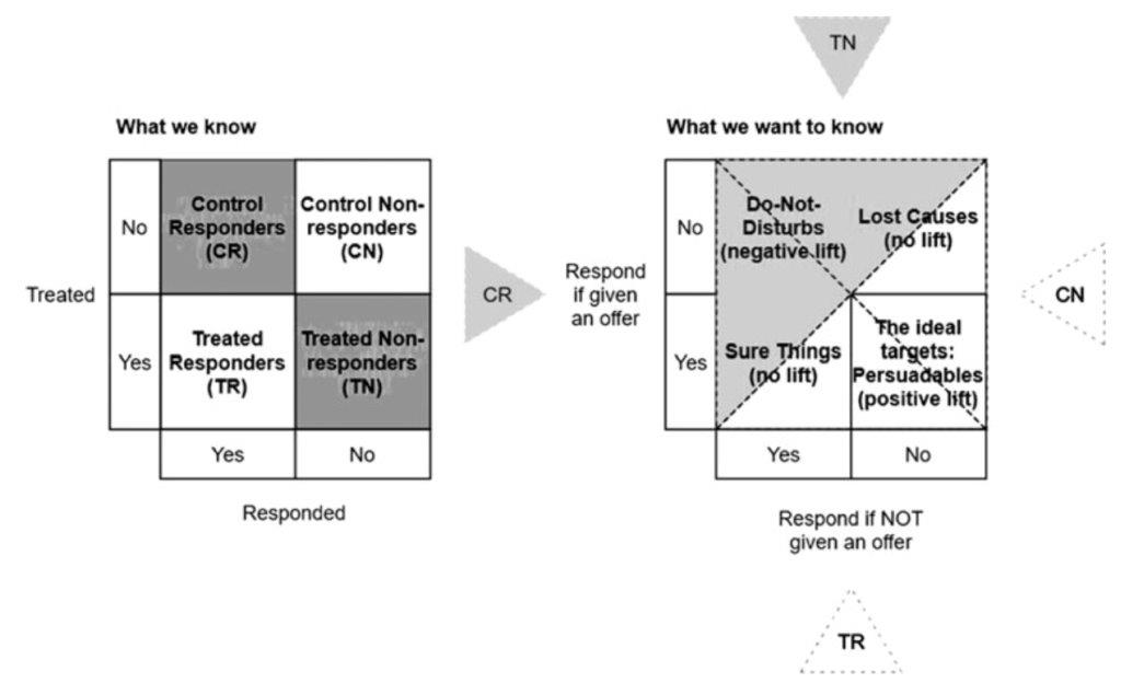
Since the group membership can not be observed individually for every customer, the class transformation method takes the information observed in the past and transforms it into a new target variable to predict group membership as best as possible. (Devriendt 2008)

What we know from previous data is whether a customer was targeted and whether the customer responded. As proposed by Lai (2006) all control nonresponders (CN) and all treatment responders (TR) are labeled as positive targets, because they contain all persuadables (customers who respond only if they are targeted). Control responders (CR) and treated nonresponders (TN) are labeled as negative targets, because they only contain do-not-disturbs (respond only when not treated), lost causes (never responds) and sure things (always respond) - groups that never create additional revenue when targeted. In this way the uplift modeling problem is transformed into a binary classification problem and the treatment effect is obtained by subtracting the probability to be negative from the probability to be positive.

$$ Uplift_{Lai}(x) = P(TR \cup CN|x) - P(TN \cup CR|x) $$

A similar approach of transforming the target variable was proposed by Jaskowski and Jaroszewicz (2012). Kane et al. (2014) further suggest a multiclass classification model to estimate each group membership separately and corrects for unequal control and treatment group sample sizes.

Two-model approach

The two-model approach is also referred to as a indirect estimation approach, because it proposes to estimate two separate predictive models for the outcome of the treatment and the control group respectively. Uplift is then determined as the difference in outcome between both models. (Devriendt 2008)

The two-model approach allows to adopt many traditional predictive modeling approaches, such as Random Forest, boosted trees or neural networks. Since both models are built and trained independently, the errors can add up when aggregating both models and lead to a poor predictive performance overall. Moreover, features that are directly related to uplift are not considered in the two-model approach, because the separate models estimate the outcome or response within the control and treatment group and not uplift directly. (Devriendt 2008)

Nevertheless, the two-model approach, especially in combination with neural networks, allows to correct for variables that impact treatment assignment in observational data. Shalit, Johansson and Sontag (2017) give a generalization-error bound to let neural networks learn a balanced representation of treatment and control distributions. Shi, Blei and Veitch (2019) introduce a new architecture, called Dragonet, which considers the treatment probability (propensity score) directly for model fitting to adjust estimations. Farrell, Liang and Misra (2019) present a neural network two-model approach, where both models are trained jointly on the whole data set. This builds also the basis for our experimental design (see section 4.3).

Modeling uplift directly

By modifying already existing machine learning algorithms, one can estimate uplift directly. Examples for tree-based approaches are provided by Radcliffe and Surry (2011), Chickering and Heckerman (2013) and Rzepakowski and Jaroszewicz (2012). Tree-based approaches mainly differ in how they modify the splitting criteria and the pruning techniques. Ensemble modeling for the estimation of individual treatment effects was for example proposed by Guleman, Guillén and Pérez-Marín (2015), who use “uplift random forests” to decrease the variance in comparison to normal decision trees. Soltys, Jaroszewicz and Rzepakowski (2015) conduct a wider analysis of ensemble approaches, focusing on bagging and random forests and conclude that ensembles provide a powerful tool for uplift modeling.

3. Descriptive Analysis of the Dataset

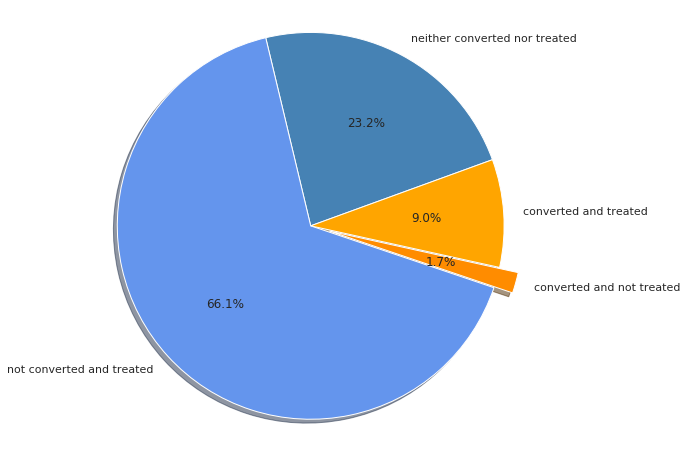
The data used for the experimental setup consists of 118,622 observations. Each observation represents a customer session in a fashion online shop. There are in total 67 different variables. The 63 features in the data set provide detailed information about the respective session, for example time and amount of views spent during each of the steps of an online purchase, device-related information, basket value or customer information. Among the features is also the treatment variable, which determines whether the customer receives an e-coupon at some point during the session which grants 10% off on the final basket value. Additionally, there are two dependant variables in the data set. The converted variable, signaling whether the customer made a purchase in the end or not, and the checkoutAmount variable, which gives to total value of the purchase. Moreover, the data set contains also the simulated treatment effects for both independent variables.

This dataset was created using A/B Test so the two assumptions mentioned before to estimate the individual treatment effect (Unconfoundedness and Overlap) are already fulfilled since the e-coupons were given out randomly.

In total, the e-coupon was offered during 75.1 % of all customer sessions. Only 10.7 % of all customer sessions ended in a purchase. But from the distribution of responders in the control and treated group one can guess that the treatment had a significant effect on the conversion. In the control group only 7 % of the sessions converted to a purchase, whereas 12 % converted in the treatment group.

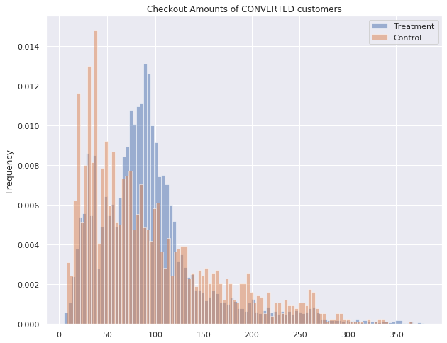
The mean checkout amount of the converted sessions is approximately 94 dollars. When considering the whole data set, the mean checkout amount drops to approximately 10 dollars because of the many non-converted sessions.

Moreover, at first sight it seems that the treatment has no direct impact on the value of the purchase. Considering only converted sessions, the mean checkout amount of the treatment group (93.60) is surprisingly lower than the mean checkout amount of the control group (94.22). But this could also be explained by other effects, for example, that treated customers that decided to buy something instead of buying nothing, will probably don’t spend as much money as customers who planned to buy something anyways.

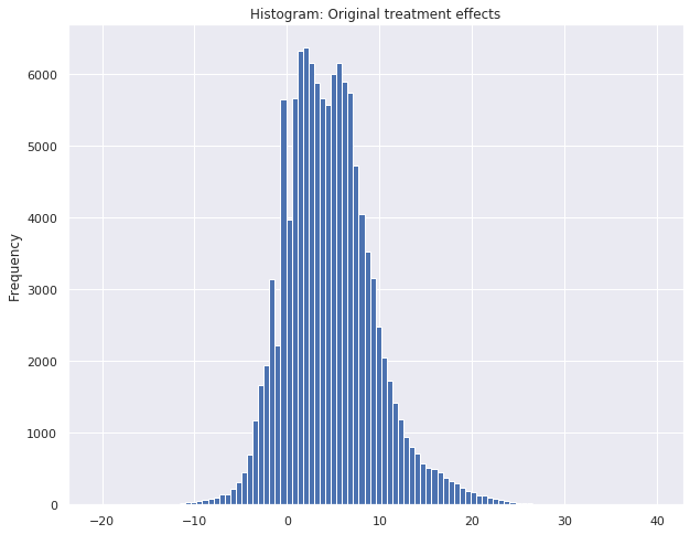
When taking a look into the simulated original treatment effects, it becomes clear that the e-coupon has an impact in the checkout amount of the customer. The mean treatment effect on the purchase value is approximately 4.6 dollars. For some sessions the treatment effect even exceeds 20 dollars, but on the other hand there are also negative treatment effects. One could assume that there are indeed customers, who do not want to be disturbed during the session and could let off from the purchase when offered an e-coupon.

4. Estimation of treatment effects considering the checkout amount

4.1 Preprocessing

Before we were able to start the actual modeling process, we had to prepare the data described above. We started separating the variables “TREATMENT EFFECT RESPONSE” and “TREATMENT EFFECT CONVERSION” from the dataset we used for training, since these variables would not appear in a real-world dataset. Anyway, having this information, we can still use it in our evaluation process to compare the computed treatment effects with the actual ones. Furthermore, for our training process we dropped the target variables “checkoutAmount” and “converted” as well as the variable “TREATMENT” of our training data. After doing so, we scaled the data, since there were some variables with values beyond the range between zero and one, which could have slowed down our training process or even make it unstable. Having this done, the data was split into a trainset (0.8), testset (0.1) and validationset (0.1). To assure, that our model makes more reliable predictions, especially when predicting the conversion of customers, we decided to balance our trainset regarding the variable conversion using undersampling. Doing so, the size of training data was reduced from 118.622 to 20.214 observations.

4.2 Benchmark Models

We got to know until this point what uplift modeling is and why are we using it. Now we’ll just present the simple equation that presents the uplift modeling, it’s known as the two-model approach (Radcliffe and Surry 2011, Lo and Pachamanova 2015), before we produce our benchmarks.

$$ f^{uplift} (X_i) = \mathbb{E}(y_i \mid x_i, T_i = 1) - \mathbb{E}(y_i \mid x_i, T_i = 0) $$

The subjects are randomized to either a treatment group (T = 1) or a control group (T = 0). We will consider only the case in which T is binary. The treatment represents the group to which some type of experimental manipulation or action is performed, and the control represents the complementary group that receives no treatment. Say we are a clothing company that would like to start a marketing campaign by giving customers 20% reductions in form of cupons. In this case the company has done it’s data analysis and found who are the customers who will get the cupons (Treatment group) and who won’t receive them (Control group). In such situations, the main interest might be in estimating the net impact of the action on an individual’s response. This is precisely the objective of uplift models. This formulation is motivated by the assumption that subjects are sensitive to the action T in different ways, and so an accurate choice of the action at the individual-subject level is essential. Even in cases when there is no global better action, in the sense that the treatment is not effective overall, there might be a subgroup of subjects for whom the treatment has positive effects, but it is being offset by negative effects on the other subgroup.

The formula above can also be presented in a shorter version, namely:

$$ \tau(x) = \mu_1 (x_i) - \mu_0 (x_i) $$

In this equation from Farrell, Liang and Misra (2019), $\tau $ is the conditional average treatment effect, $ \mu_1 $ is the spending of the customer when he is treated and $ \mu_0 $ is the spending of the customer when he is not treated.

One way to solve this equation (and the problem at hand) is by building two separate models one for the treatment group (to predict $ \mu_1 $) and one for the control group (to predict $ \mu_0 $) and then subtract the estimated value of response from the two models. The two-model approach has the significant benefit of being straightforward to implement and allowing to adopt traditional predictive modeling approaches, such as Linear Regression, Logistic Regression, Decision Trees, Random Forests and Neural Networks. We will explain briefly the two predictive models we chose as a benchmark for our paper.

• Random Forest

Tree-based models are a natural approach to estimate the presented equation, because they partition the input space into segments, and appropriate split criteria can be designed to model uplift directly. In their paper Rzepakowski and Jaroszewicz (2012) they proposed what is believed by many in the uplift literature to be the the most sensible split criteria because they are supported by well-known measures of distributional divergence from the information theoretic literature. This is also the recommended approach for standard decision trees. The only “problem” if we are allowed to name it that way is that their model was based on a single tree. One of the main problems with trees is their high variance that is generated from the hierarchical way of the splitting process, in other words the effect of an error in the top split is propagated down to all of the splits below. There are two ways to tackle this problem to lighten the variance one of them is bagging methods introduced by (Breiman 1996). This will improve the stability but it’s limited still. The second solution is Random Forest which improves the variance reduction of the bagging methods. There are two types of Random Forest which are:

1. Regressor which we use for the estimation of treatment effects considering the checkout amounts
2. Classifier which we use for the estimation of treatment effects considering the conversion

• Linear Regression

Linear regression is one of the many regression methods available. Regression searches for relationships among variables. For example, we can look at our dataset and observe each customer and try to find out how the checkout amount that is presented in the dataset is affected by the other features presented as well (when the customer visited the website, from what device and at what time, etc). Generally, in regression analysis, you usually consider some phenomenon of interest and have a number of observations. Each observation has two or more features. Following the assumption that (at least) one of the features depends on the others, you try to establish a relation among them. In other words, you need to find a function that maps some features or variables to others sufficiently well.

• Logistic Regression

Logistic regression is one of the many used machine learning algorithms for binary classification problems, which are problems with two class values, including predictions such as “yes or no”. It predicts a dependent data variable by analyzing the relationship between one or more existing independent variables. For example, a logistic regression could be used to predict whether (in our case) a customer will respond to our offer or not. The model resulted from this can take into consideration many input variables such as when the customer visited the website, from what device and at what time, etc. Based on older data that we obtain about earlier outcomes involving the same input variables, the model will now score new cases on their possibilities of falling in one of the two categories we have (respond to the offer or not).

• Neural Network

Also referred to as Artificial Neural Network (ANN)or just neural net, it’s obvious the concept was inspired from human biology and the way neurons of the human brain function together to understand inputs from human senses. Neural networks are typically organized in layers. Layers are made up of a number of interconnected ‘nodes’ which contain an ‘activation function’. Patterns are presented to the network via the ‘input layer’, which communicates to one or more ‘hidden layers’ where the actual processing is done via a system of weighted ‘connections’. The hidden layers then link to an ‘output layer’ where the results (usually the predictions) are delivered back. A neural network is a set of algorithms that tries to identify underlying relationships in a set of data. They do this using a process that mimics the way our brain operates. Neural networks can learn in one of three different ways:

• Supervised Learning: a set of inputs and outputs are fed to the algorithms. They then predict the outcomes after being trained on how to interpret the data.
• Unsupervised Learning: the learning occurs without human help. The algorithms use data that is neither labeled nor classified. They act on that data without guidance.
• Reinforcement Learning: this involves taking suitable action to maximize reward in a particular situation. The algorithms learn, depending on the feedback you give them. This is a bit like helping someone find something by telling them whether they are getting warmer or colder.

Evaluation Metrics

The evaluation metrics that can be used differ depending on the model created. As we know models can be classified as classification or regression models. Using more than one evaluation metric is advised because a model can perform really good on one metric and then not so good on another metric. Since we do have the actual treatment effects in our data and we are able to use them for evaluation, the metrics used for our regression models are the:

1. Mean absolute error:

This metric calculates the difference between the predicted value and the actual value by subtraction and this represents the errors. “absolute” is because we convert each error to positive by taking it’s absolute value and “mean” it looks for the average of a set of errors.

2. Mean squared error:

Just like Mean absolute error, the errors are represented by the difference between the actual and predicted values. “squared” comes from the fact that this metric squares all the “differences” in order to avoid having negative values, it also gives more weight to larger “differences”. the “mean” is because it looks for the average of a set of errors.

4.2.1 Data preparation for the Two Model Approach

As described above, the Residual model which will be introduced in chapter 4.3 will be compared to other models using the two model approach. Since two different models need to be trained on the data of the treated group (to predict $\mu_1$) or on the data of the control group (to predict ($ \mu_0 $), the dataset has to be split into these two groups.

4.2.2 Random Forest Regressor - Two Model Approach

We built two Random Forests Regressors, one for the treatment group and one for the control group, the parameters were chosen after running hyper parameter optimization. Afterwards we fitted them and trained them separately and at the end we subtracted the predictions of the control group from the predictions of the treatment group to estimate the individual treatment effect as you can see in the code below.

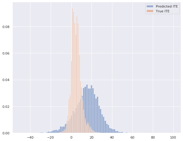
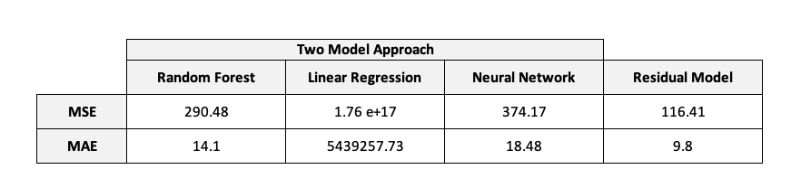
As we can see in the histogram beneath, our random forest regressor model seems to be able to predict individual treatment effects that are somewhat close to the true treatment effects. This model has a mean absolute error of 14.10 and a mean squared error of 290.48.

4.2.3 Linear Regression - Two Model Approach

In this approach we might think it’s performing similar to the previous model by looking at the histogram but in reality it isn’t. This model has a mean absolute error of 5439257.73 and a mean squared error of 1.76e+17 and the reason for that is because it’s predicting some extremely negative values.

4.2.4 Neural Network - Two Model Approach

As we decided to use pytorch to build our model to be more flexible in adapting it later on, we had to define our class for the neural network. To be able to build different types of models with the same class, it was implemented in a way that the number of layers can be given as an input with the number of nodes for the single layers. So when creating the model, linear layers are created. In the forward function that is used, these linear layers are always connected with a relu function and the output layer is a linear layer.

After building the class, two models, one for the treatment and one for the control group are built.

These models (only nn_treat shown here) are then trained for 50 epochs using the function below.

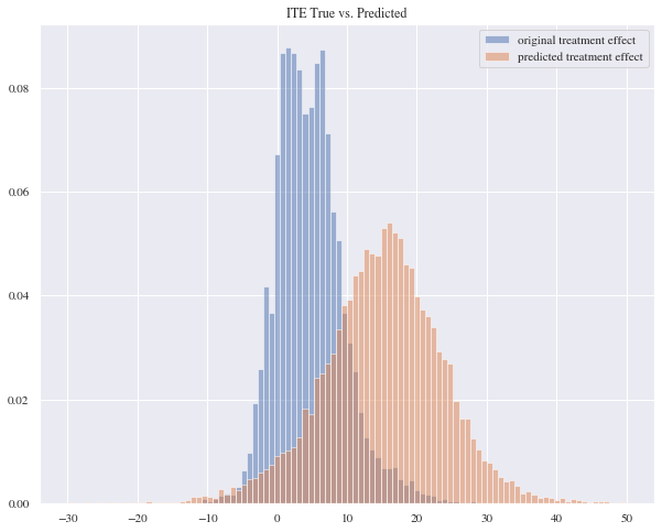
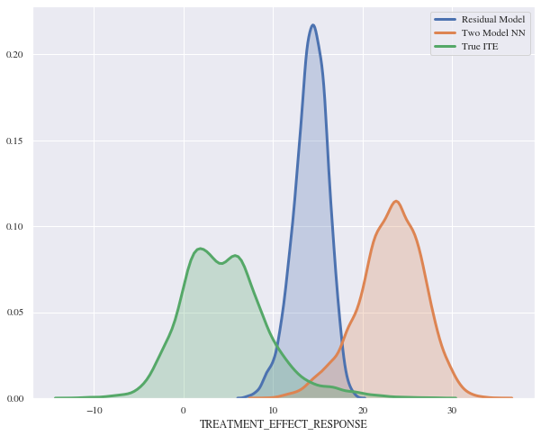
It seems that the true treatment effects and the predicted ones don’t match but they almost have identical distribution curves. The mean absolute error for this model is 18.48 and the mean squared error is 374.17.

4.3 Residual Model

4.3.1 Theory

Using and training two models for predicting one value comes with much computation and many lines of code. Inspired by Farrell, Liang and Misra (2019), we tried to implement a model, where all data from the treatment and control group can be used in one training process. Therefore, we will again have a look at the formula we already mentioned before:

$$ \tau(x_i) = \mu_1 (x_i) - \mu_0 (x_i) $$

One can see by converting the formula, that the spendings of a treated customer ($ \mu_1 $) is equal to the sum of the spendings of the customer without treatment ($ \mu_o $) and his individual treatment effect ($ \tau $).

$$ \mu_1 (x_i) = \mu_0 (x_i) + \tau(x_i) $$

So we implemented our model in a way, that $ \mu_o $ and $ \tau(x) $ were trained jointly. For that, we implemented a model consisting of two other models. One model (nn_base) is trained to predict $ \mu_o $, so this is the part of the model which is active for every observation passed through the model, regardless of whether the customer was treated or not. The second part of the model takes advantage of the fact, that a person is either treated ($ T = 1 $) or not treated ( $ T=0 $ ). So we used this binary parameter to add the second part to the Residual model, which estimates the individual treatment effect $ \tau (x_i) $. This part is represented by another model (nn_ite) and is only active, if the customer was treated. If the customer was not treated, only the nn_base model is used for the prediction.

So generally spoken, our Residual model predicts the spending of the customer, based on his individual characteristics ($x_i$) and on the binary variable $T$, giving the model the information, whether the customer was treated or not.

In a more formal way, the model prediction is calculated as follows:

$$ \mu_1 (x_i, T_i) = \mu_0 (x_i) + T_i * \tau(x_i) $$

Besides the fact, that this saves a lot of code for separating the data into a treatment and a control group, as well as only one model needs to be trained, this model comes with another advantage. After training the Residual model, that predicts the customers spending, we do also have the model nn_ite predicting the treatment effect. Hence, we can use this model to predict the treatment effect for a customer and do not have to subtract different models as we have seen in the benchmark modeling part above.

Additionally, in the application of Farrell, Liang and Misra (2019), the joint training outperformed the separate estimation of $ \mu_o $ and $ \mu_1 $, even though these approaches are equivalent theoretically.

4.3.2 Implementation

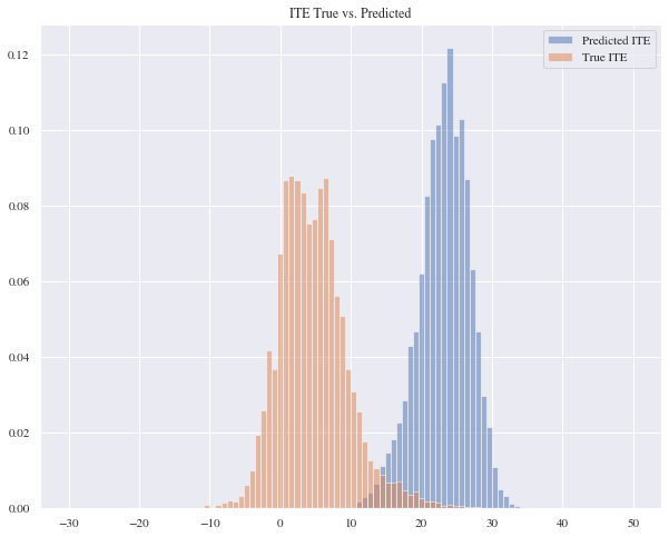
This model outperforms the benchmarks we presented before and the evaluation metrics scores also support this evidence since its scored 9.80 for the mean absolute error and 116.41 for the mean squared error.

4.4 Summary Treatment Effects considering the checkout amount

Even though the histogram for the regression looked promising, some extremely negative predictions lead to tremendously bad scores for the mean absolute error and mean squared error. Besides that, the large difference between the two model approach for the neural network and the Residual model was surprising, since they are equivalent theoretically.

When comparing the results from the two model approach and the Residual model that are both using a neural network structure, one can see that the predictions of the Residual model are more precise than the ones from the two model approach. This was also observed by Farrell, Liang and Misra (2019). One possible reason for that could be the fact, that it may be difficult to predict the basket values for both models, hence the errors might add up in the end. Showing this in equations:

• nn_control predicts: $$\mu_0 (x_i) + error_{control}$$
• nn_treated predicts: $$\mu_1 (x_i) + error_{treated}$$

So with these errors, our predicted treatment is:

$$ \tau(x_i) = (\mu_1 (x_i) + error_{treated}) - (\mu_0 (x_i) + error_{control}) $$

So in worst case, when adding up the models, $error_{treated}$ could be positive and error_{control} could be negative, which would reduce the calculated treatment effect significantly, or the other way around enlarge it. It seems like training $\mu_0 (x_i)$ and $ \tau(x_i)$ jointly reduces the total error.

This is, because the model for the treatment effect tries to predict the whole difference between the predicted value for $\mu_0$ and the actual value. So in the end, the part of our Residual model that predicts the treatment effect includes also this error of the first model predicting $\mu_0$.

$$ \mu_1 (x_i, T_i) = \mu_0 (x_i) + T_i * \tau(x_i) $$

Comparing the results from our Residual model to the benchmark models shows that the Residual model clearly outperforms all of them, especially regarding the mean absolute error (9.80) and mean squared error (116.41).

5. Estimation of Treatment Effects considering conversion

5.1 Benchmark Models

Evaluation Metrics

Until this point, we were dealing with the individual treatment effects regarding the checkout amounts. In the following part of the blogpost, we are going to predict the individual treatment effects considering the conversion of a customer. So we will try to estimate, how the treatment of a customer with a coupon is changing its probability to buy something in the end. Even though predicting, whether a customer is going to convert or not is a classification problem, the prediction of the treatment effects is still a regression problem. So although we are building two different classification models when we are using our two model approach, in the end we are still evaluating our Individual Treatment Effects which is regression problem so we are going to use the metrics provided before which are Mean absolute error and Mean squared error. In addition we are going to present a new evaluation metrics called Qini curves since it can be used in real world data where we don’t actually have any treatment effect values given.

1. Qini curves:

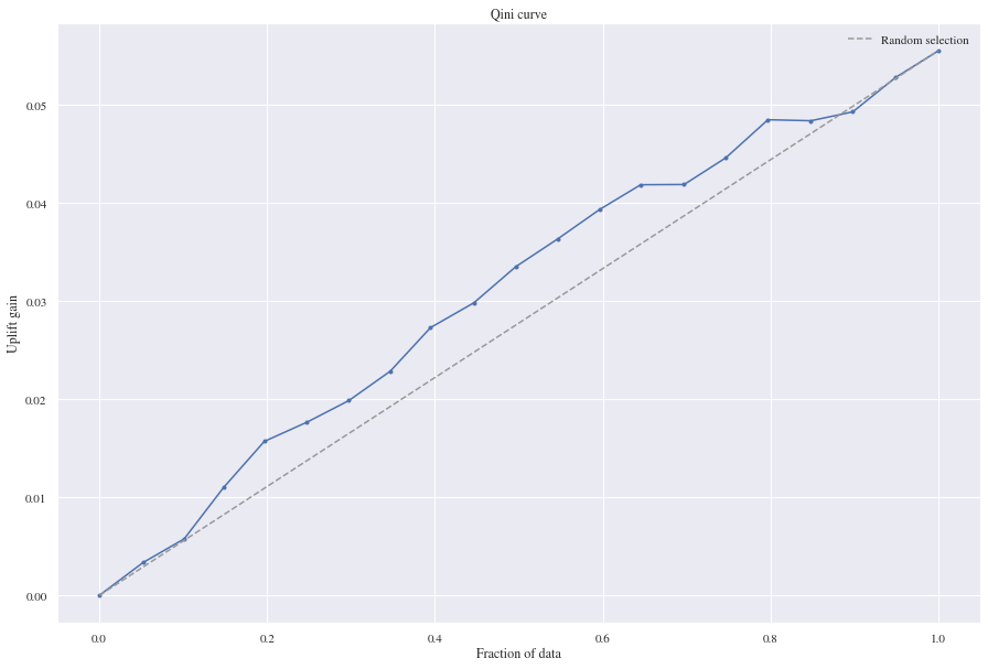
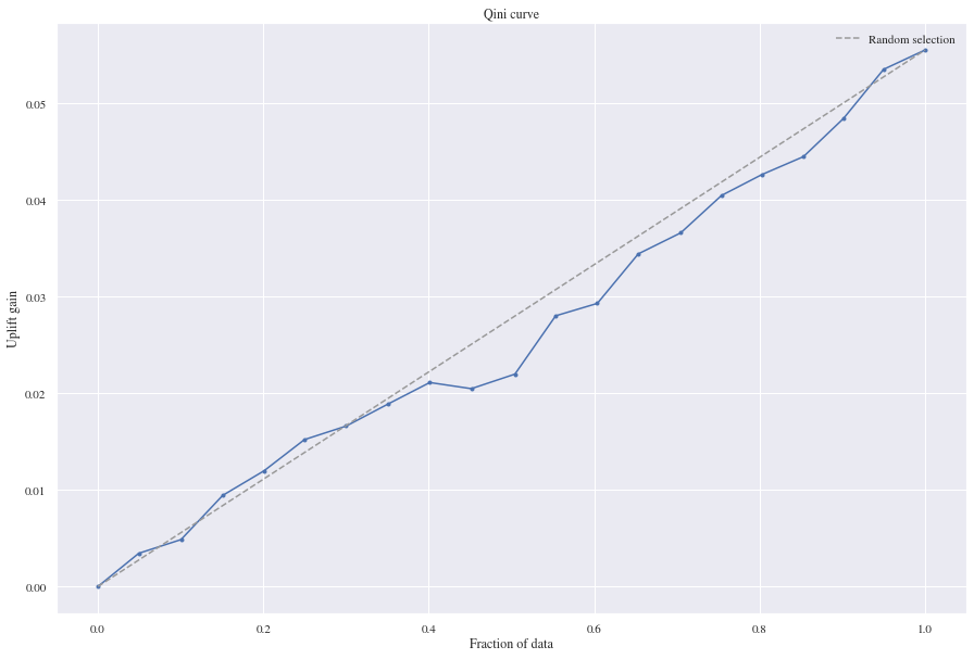
An evaluation metric for uplift models are the Qini curves which can be viewed as an extension to the corresponding gini coefficient and the cumulative gain charts which help assess a response model (Radcliffe). In standard lift metric, gain is defined as the number of conversions for response models or the value of these conversions for revenue models. So what is the difference between Qini and Gini? an estimate of Gini is obtained on a graph of a conventional gain curve (Y = number of responses), the Qini coefficient is measured on the uplift curve (Y = incremental gain). Qini remains simply a variation of Gini, the main difference being Qini is a specialized measure of the AUUC (area under uplift curve) while Gini is a broader measurement of AUC. The Qini curve of a model is compared to a random model. The performance line of the random model starts in the coordinate system’s origin and ends in a point that represents the total population size and the total incremental number of purchases (conversion modeling) or total incremental revenue (revenue modeling) (This is again according to Radcliffe).The Qini values is defined as the area between the model gain curve and the random model (diagonal line). In our code we used a package called “pylift” which is an already programmed package that can help us in plotting our Qini curves.

5.1.1 Random Forest Classifier - Two Model Approach

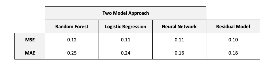
We trained the two random forest classifiers to predict probabilities instead of classes to be able to examine treatment effects. When we are having a look at the results the Random Forest Classifier is performing good on the Qini curve since there’s gain on the uplift and it has a mean squared error of 0.12 and a mean absolute error of 0.25.

5.1.2 Logistic Regression - Two Model Approach

For the Logistic regression model we did also predict probabilities for the single models to be able to calculate the treatment effects. The two model logistic regression approach didn’t perform good on the Qini curve since the uplift gains that we can get from the random model were higher than our benchmark. This model’s mean squared error 0.11 and mean absolute error 0.24.

5.1.3 Neural Network - Two Model Approach

Having a look at the two model approach using two neural nets, we see that the approach is gaining a bit more uplift than the random model and is actually performing good on the evaluation metrics we’re using. It scored a mean squared error of 0.11 and a mean absolute error of 0.16.

5.2 Residual Model - Classification

5.2.1 Theory

As shown above, the approach using only one model to predict the individual treatment effects worked. Facing a classification problem, this model architecture comes with a weakness, as the results of two models are added up together.

$$ \mu_1 (x_i, T_i) = \mu_0 (x_i) + T_i * \tau(x_i) $$

For our classification problem it could be possible, that a customer already has a high probability to buy the product ($\mu_0$), even if he is not treated. Nevertheless, he could also be very receptive to advertisement and hence treating him could lead to a large individual treatment effect ($\tau$). In this case, predicting the probability that the customer buys the product could lead to a value larger than 1 for $\mu_1$. Since the maximum probability of an event to happen is 1 and it is not possible, that a customer buys something with a probability larger than 1, we need to adapt our model for this special task.

So the idea is to make use of the sigmoid function, which has the nice feature of bringing the results into a range from 0 to 1. For this reason we wrapped the sum of the models for $\mu_0$ and $\tau$ into a sigmoid function to avoid having results larger than 1 for $\mu_1$.

$$ \mu_1 (x_i, T_i) = sig(\mu_0 (x_i) + T_i * \tau(x_i)) $$

5.2.2 Implementation

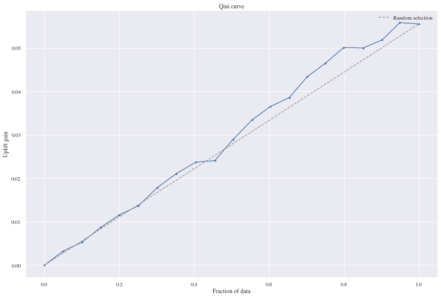
From the Qini curve we can see that our Residual model gained some uplift and predicted better than the random model. 0.10 is the registered mean squared error and 0.18 is the mean absolute error.

5.3 Summary Treatment Effects considering conversion

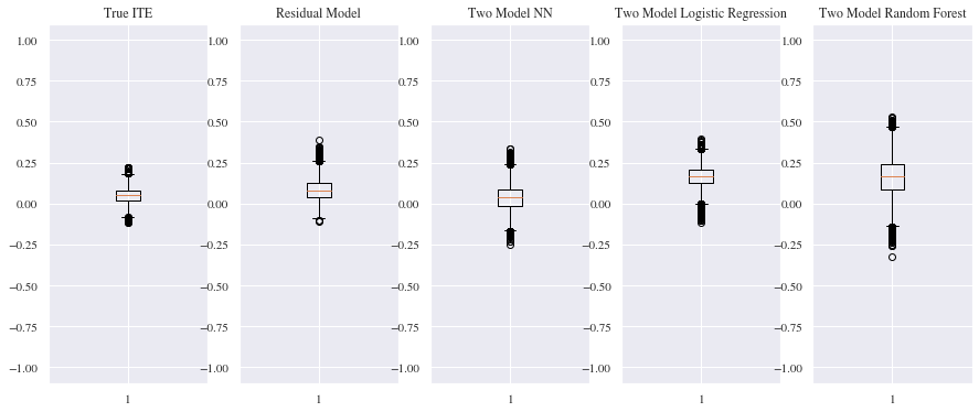
Comparing the results of the benchmark models with the Residual approach we can see that all of them are close to each other concerning the MSE and MAE. Nevertheless, for MSE the Residual model performs slightly better than the benchmark models. Both neural networks models, the Residual and the two model approach, are performing better than the two other models on the MAE with the two model approach neural network having a slight advantage. From the boxplot below we can tell that the mean of the predicted individual treatment effect for our validation data is around 0.05 and the logistic regression and the random forest seem to have overestimated the treatment effect. For the Residual model the mean of the estimated treatment effects is slightly above the true individual treatment effect while the two model neural network approach seems to underestimate the treatment effect.

Even though the result of the Residual model are looking very promising,the values might differ from the actual individual treatment effects, as for the prediction only the second model nn_ite that was trained to predict the treatment effects during the training of the residual model was used for the predictions. Since both models in the residual model were wrapped into the sigmoid function, using the models predictions without passing them through the sigmoid function might also change the values of the treatment effects.

6. Placebo Experiment

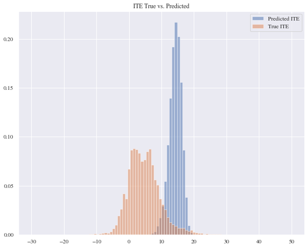
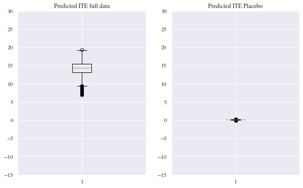
To examine, whether our model really is able to detect causal effects, we did a placebo experiment as described in Farrell, Liang and Misra (2019). So for the test, we selected all customers without a treatment and randomly assigned them to a group $T=0$ or $T=1$, which is our placebo group in this experiment. Afterwards the residual model was again trained on predicting the individual treatment effect considering the checkout amount. One can see easily in the plot beneath on the right side, that the Residual model that was trained on the placebo group examined, that there was no treatment effect. For comparison, on the left side again the estimated treatment effects from part 4 are shown.

7. Conclusion

In this blogpost, we gave a brief literature overview about the topic of uplift modeling and treatment effects. We then described the dataset used for the tests of the residual model. We trained the Residual model on two different tasks, namely the estimation of treatment effects considering the checkout amount of a customer, and estimating the individual treatment effects considering the probability of a customer to finally buy something (conversion). As a benchmark for the residual model, we used the two model approach using the Random Forest Regressors, Linear Regression models, Neural Networks (for the basket values) and Random Forest Classifiers, Logistic Regression models and also Neural Networks.

For the first task (estimation of treatment effects considering the checkout value) the Residual Model outperformed the other models concerning the MSE and MAE. There was a difference between the Two Model Neural Network approach and the Residual Model, even though they are equivalent theoretically. One possible reason for that was shown with the prediction errors, but there might be other explanations for that as well. Additionally we observed, that the treatment effects of the two model approach seemed to be shifted away from the actual treatment effects. For future research, it could be interesting to set up the residual model not only with neural networks but also with other models, as there might be some patterns in the difference between Two Model Approach and Residual Model using the same models, as we have seen for our neural networks.

In the second task the results of the Two Model Approach using Neural Networks and the Residual Model were more similar. Concerning the MSE, the Residual Model performed best, while having a look at the MAE the Two Model Neural Network Approach got the best score. Even though both of the models were close to the true treatment effects when we were having a look at their distribution, one should keep in mind, that the extraction of the treatment effects for the Residual Model using the Sigmoid function could lead to some deviations. In a next step, one could think about extracting the individual treatment effects of the model using the reverse function of Sigmoid or another solution to avoid these possible deviations. Furthermore, the Residual Model could be tested on other datasets.

In the last part of our blogpost, to prove that the Residual Model really examines individual treatment effects, we showed a placebo experiment, where we trained the Residual Model on a dataset where no customer was treated. In this experiment it was shown, that the model in this case was not able to find any treatment effects as there were none.

All in all, the Residual Model seems to perform good and worked better than our benchmark models. Additionally it comes with the advantage of having only one model to predict a treatment effect when the model was finally trained.

References

Chickering, D. M. and Heckerman, D. (2013). A decision theoretic approach to targeted advertising. arXiv preprint arXiv:1301.3842.

Devriendt, F., Moldovan, D., and Verbeke, W. (2018). A literature survey and experimental evaluation of the state-of-the-art in uplift modeling: A stepping stone toward the development of prescriptive analytics. Big data, 6(1):13-41. 10

Diemert, E., Betlei, A., Renaudin, C., and Amini, M-R. (2018). A Large Scale Benchmark for Uplift Modeling. In AdKDD Workshop.

Farrell, M. H., Liang, T., and Misra, S. (2019). Deep neural networks for estimation and inference. arXiv preprint arXiv:1809.09953.

Guelman, L., Guillen, M., and Perez-Marn, A. M. (2015). Uplift random forests. Cybernetics and Systems, 46(3-4):230-248.

Gutierrez, P. and Gerardy, J.-Y. (2017). Causal inference and uplift modelling: A review of the literature. In International Conference on Predictive Applications and APIs, pages 1-13.

Haupt, J., Jacob, D., Gubela, R. M., and Lessmann, S. (2019). Affordable uplift: Supervised randomization in controlled experiments. Fortieth International Conference on Information Systems.

Imbens, G. W. and Wooldridge, J. M. (2009). Recent developments in the econometrics of program evaluation. Journal of economic literature, 47(1):5-86.

Jaskowski, M. and Jaroszewicz, S. (2012). Uplift modeling for clinical trial data. In ICML Workshop on Clinical Data Analysis.

Kane, K., Lo, V. S., and Zheng, J. (2014). Mining for the truly responsive customers and prospects using true-lift modeling: Comparison of new and existing methods. Journal of Marketing Analytics, 2(4):218-238.

Lai, L. Y.-T. (2006). Influential marketing: a new direct marketing strategy addressing the existence of voluntary buyers. PhD thesis, School of Computing Science-Simon Fraser University.

Radcliffe, N. J. and Surry, P. D. (2011). Real- world uplift modelling with significance-based uplift trees. White Paper TR-2011-1, Stochastic Solutions, pages 1-33.

Rudas, K. and Jaroszewicz, S. (2018). Linear regression for uplift modeling. Article in Data Mining and Knowledge Discovery.

Rzepakowski, P. and Jaroszewicz, S. (2012). Decision trees for uplift modeling with single and multiple treatments. Knowledge and Information Systems, 32(2):303-327.

Shalit, U., Johansson, F. D., and Sontag, D. (2017). Estimating individual treatment effect: generalization bounds and algorithms. In Proceedings of the 34th International Conference on Machine Learning- Volume 70, pages 3076-3085. JMLR. org. 11

Shi, C., Blei, D., and Veitch, V. (2019). Adapting neural networks for the estimation of treatment effects. In Advances in Neural Information Processing Systems, pages 2503-2513.

Soltys, M., Jaroszewicz, S., and Rzepakowski, P. (2015). Ensemble methods for uplift modeling. Data mining and knowledge discovery, 29(6):1531-1559.