By Seminar Information Systems (WS19/20) | February 6, 2020
Deep Learning for Survival Analysis
Authors: Laura Löschmann, Daria Smorodina
Table of content
- Motivation - Business case
- Introduction to Survival Analysis
- Dataset
- Standard methods in Survival Analysis
- Deep Learning for Survival Analysis
- Evaluation
- Conclusion
- References
1. Motivation - Business case
With the financial crisis hitting the United States and Europe in 2008, the International Accounting Standards Board (IASB) decided to revise their accounting standards for financial instruments, e.g. loans or mortgages to address perceived deficiencies which were believed to have contributed to the magnitude of the crisis.The result was the International Financial Reporting Standard 9 that became effective for all financial years beginning on or after 1 January 2018 [1].
Previously impairment losses on financial assets were only recognised to the extent that there was an objective evidence of impairment, meaning a loss event needed to occur before an impairment loss could be booked [2]. The new accounting rules for financial instruments require banks to build provisions for expected losses in their loan portfolio. The loss allowance has to be recognised before the actual credit loss is incurred. It is a more forward-looking approach than its predecessor with the aim to result in a more timely recognition of credit losses [3].
To implement the new accounting rules banks need to build models that can evaluate a borrower’s risk as accurately as possible. A key credit risk parameter is the probability of default. Classification techniques such as logistic regression and decision trees can be used in order to classify the risky from the non-risky loans. These classification techniques however do not take the timing of default into account. With the use of survival analysis more accurate credit risks calculations are enabled since these analysis refers to a set of statistical techniques that is able to estimate the time it takes for a customer to default.
2. Introduction to Survival Analysis
Survival analysis also called time-to-event analysis refers to the set of statistical analyses that takes a series of observations and attempts to estimate the time it takes for an event of interest to occur.
The development of survival analysis dates back to the 17th century with the first life table ever produced by English statistician John Graunt in 1662. The name “Survival Analysis” comes from the longstanding application of these methods since throughout centuries they were solely linked to investigating mortality rates. However, during the last decades the applications of the statistical methods of survival analysis have been extended beyond medical research to other fields [4].
Survival Analysis can be used in the field of health insurance to evaluate insurance premiums. It can be a useful tool in customer retention e.g. in order to estimate the time a customer probably will discontinue its subscription. With this information the company can intervene with some incentives early enough to retain its customer. The accurate prediction of upcoming churners results in highly-targeted campaigns, limiting the resources spent on customers who likely would have stayed anyway. The methods of survival analysis can also be applied in the field of engineering, e.g. to estimate the remaining useful life of machines.
2.1 Common terms
Survival analysis is a collection of data analysis methods with the outcome variable of interest time to event. In general event describes the event of interest, also called death event, time refers to the point of time of first observation, also called birth event, and time to event is the duration between the first observation and the time the event occurs [5]. The subjects whose data were collected for survival analysis usually do not have the same time of first observation. A subject can enter the study at any time. Using durations ensure a necessary relativeness [6]. Referring to the business case the birth event is the initial recognition of a loan, the death event, consequently the event of interest, describes the time a customer defaulted and the duration is the time between the initial recognition and the event of default.
During the observation time not every subject will experience the event of interest. Consequently it is unknown if the subjects will experience the event of interest in the future. The computation of the duration, the time from the first observation to the event of interest, is impossible. This special type of missing data can emerge due to two reasons:
- The subject is still part of the study but has not experienced the event of interest yet.
- The subject experienced a different event which also led to the end of study for this subject.
In survival analysis this missing data is called censorship which refers to the inability to observe the variable of interest for the entire population. However, the censoring of data must be taken into account, dropping unobserved data would underestimate customer lifetimes and bias the results. Hence the particular subjects are labelled censored.
Since for the censored subjects the death event could not be observed, the type of censorship is called right censoring which is the most common one in survival analysis. As opposed to this there is left censoring in case the birth event could not be observed.
The first reason for censored cases regarding the use case are loans that have not matured yet and did not experience default at the moment of data gathering.
The second reason for censorship refers to loans that did not experience the event of default but the event of early repayment. With this the loan is paid off which results in the end of observation for this loan. This kind of censoring is used in models with one event of interest [7].
In terms of different application fields an exact determination of the birth and death event is vital. Following there are a few examples of birth and death events as well as possible censoring cases, besides the general censoring case that the event of interest has not happened yet, for various use cases in the industry:

2.2 Survival function
The set of statistic methods related to survival analysis has the goal to estimate the survival function from survival data. The survival function $S(t)$ defines the probability that a subject of interest will survive beyond time $t$, or equivalently, the probability that the duration will be at least $t$ [8]. The survival function of a population is defined as follows:
$$S(t) = Pr(T > t)$$
$T$ is the random lifetime taken from the population under study and cannot be negative. With regard to the business case it is the amount of time a customer is able to pay his loan rates, he is not defaulting. The survival function $S(t)$ outputs values between 0 and 1 and is a non-increasing function of $t$.
At the start of the study ($t=0$), no subject has experienced the event yet. Therefore the probability $S(0)$ of surviving beyond time zero is 1. $S(\infty) = 0$ since if the study period were limitless, presumably everyone eventually would experience the event of interest and the probability of surviving would ultimately fall to 0. In theory the survival function is smooth, in practice the events are observed on a concrete time scale, e.g. days, weeks, months, etc., such that the graph of the survival function is like a step function [9].
![(Source: [9a])](http://blog/img/seminar/group2_SurvivalAnalysis/survival_function.png)
(Source: [9a])
2.3 Hazard function
Derived from the survival function the hazard function $h(t)$ gives the probability of the death event occurring at time $t$, given that the subject did not experience the death event until time $t$. It describes the instantaneous potential per unit time for the event to occur [10].
$$h(t) = \lim_{\delta t\to 0}\frac{Pr(t \leq T \leq t+\delta t | T>t)}{\delta t}$$
Therefore the hazard function models which periods have the highest or lowest chances of an event. In contrast to the survival function, the hazard function does not have to start at 1 and go down to 0. The hazard rate usually changes over time. It can start anywhere and go up and down over time. For instance the probability of defaulting on a mortgage may be low in the beginning but can increase over the time of the mortgage.
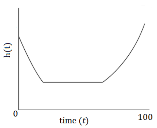 (Source: [10a])
The above shown graph is a theoretical example for a hazard function [11]. This specific hazard function is also called bathtub curve due to its form. This graph shows the probability of an event of interest to occur over time.
It could describe the probability of a customer unsubscribing from a magazine over time. Within the first 30 days the risk to unsubscribe is high, since the customer is testing the product. But if the customer likes the content, meaning he “survives” the first 30 days, the risk of unsubscribing decreased and stagnates at lower level. After a while the risk is increasing again since the customer maybe needs different input or got bored over time. Hence the graph gives the important information when to initiate incentives for those customers whose risk to unsubsribe is about to increase in order to retain them.
The main goal of survival analysis is to estimate and interpret survival and/or hazard functions from survival data.
3. Dataset
We used the real-world dataset of 50.000 US mortgage borrowers which was provided by International Financial Research (www.internationalfinancialresearch.org). The data is given as a “snapshot” in a panel format and represents a collection of US residential mortgage portfolios over 60 periods. Loan can originate before the initial start of this study and be paid after it will be finished as well.
When a person applies for mortgage, lenders (banks) want to know the value of risk they would take by loaning money. In the given dataset we are able to inspect this process using the key information from the following features:
- Various timestamps for loan origination, future maturity and first appearance in the survival study.
- Outside factors like gross domestic product (GDP) or unemployment rates at observation time.
- Average price index at observation moment.
- FICO score for each individual: the higher the score, the lower the risk (a “good” credit score is considered to be in the 670-739 score range).
- Interest rates for every issued loan.
- Since our object of analysis is mortgage data we have some insights for inquired real estate types (home for a single family or not, is this property in area with urban development etc.) which are also playing an important role for prospective loan amount.
In order to use our data for survival analysis, we need to specify the characteristic terms. The birth event is the time of the initial recognition of the mortgage, the death event is the default of the customer. The duration is the time between the birth and death event. Some customers have not defaulted yet, so they will be labelled “censored” in further analysis.
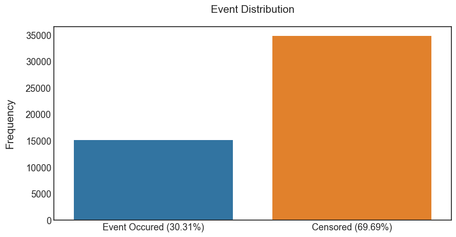
The graph below shows an example for the censorship concept at specific point in time (13 months).

Some customers defaulted before this point in time (red lines) and some “survived” beyond it (marked with blue lines) and at this point in time it is unknown if these customers will experience the event of interest.
Handling this kind of the missing information is a main advantage of survival analysis. The distribution of the event of interest (in graph below) shows that more than 2/3 of customers are labelled as “censored”. Dropping out these observations would lead to a significant information loss and a biased outcome.
Survival analysis requires a specific dataset format:
- $E_i$ is the event indicator such that $E_i = 1$, if an event happens, and $E_i = 0$ in case of censoring (column default_time)
- $T_i$ is the observed duration (total_obs_time column)
- $X_i$ is a $p$−dimensional feature vector (covariates starting from the third column).

4. Standard methods in Survival Analysis
The standard ways for estimation can be classified into the three main groups: non-parametric, semi-parametric, and parametric approaches. The choice which method to use should be guided by the dataset design and the research question of interest. It is feasible to use more than one approach.
- Parametric methods rely on the assumptions that the distribution of the survival times corresponds to specific probability distributions. This group consists of methods such as exponential, Weibull and lognormal distributions. Parameters inside these models are usually estimated using certain maximum likelihood estimations.
- In the non-parametric methods there are no dependencies on the form of parameters in underlying distributions. Mostly, the non-parametric approach is used to describe survival probabilities as function of time and to give an average view of individual’s population. The most popular univariate method is the Kaplan-Meier estimator and used as first step in survival descriptive analysis (section 4.1).
- To the semi-parametric methods corresponds the Cox regression model which is based both on parametric and non-parametric components (section 4.2).
Generally, the range of available statistical methods which can be implemented in survival analysis is very extensive and a selection of them is introduced in the scope of our blog post. The diagram below helps to briefly familarize with them:
![(Source: [18])](group2_SurvivalAnalysis/overall1.jpg)
(Source: [18])
4.1 Kaplan - Meier estimator
The key idea of the Kaplan-Meier estimator is to break the estimation of the survival function $S(t)$ into smaller steps depending on the observed event times. For each interval the probability of surviving until the end of this interval is calculated, given the following formula:
$$ \hat{S(t)} = \prod_{i: t_i <= t}{\frac{n_i - d_i}{n_i}} ,$$ where $n_i$ is a number of individuals who are at risk at time point $t_i$ and $d_i$ is a number of subjects that experienced the event at time $t_i$.
When using Kaplan-Meier estimator, some assumptions must be taken into account:
- All observations - both censored and defaulted - are used in estimation.
- There is no cohort effect on survival, so the subjects have the same survival probability regardless of their nature and time of appearance in study.
- Individuals who are censored have the same survival probabilities as those who are continued to be examined.
- The survival probability is equal for all subjects.
The main disadvantage of this method is that it cannot estimate survival probability considering all covariates in the data (it is an univariate approach) which shows no individual estimations but the overall population survival distribution. In comparison, semi- and parametric models allow to analyse all covariates and estimate $S(t)$ with respect to them.
The estimated $S(t)$ can be plotted as a stepwise function of overall population of individuals. As an example, in the plot below, it is clear that for time $t = 10$ months the probability that borrowers survive beyond this time is about 75%.

4.2 Cox proportional hazards Model
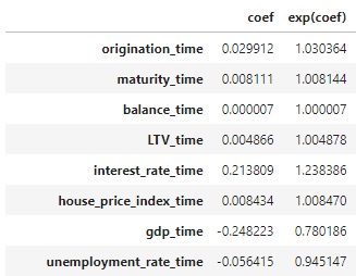
The Cox proportional hazards model (CoxPH) involves not only time and censorship features but also additional data as covariates (for our research all features of the dataset were used).
The Cox proportional hazards model (1972) is widely used in multivariate survival statistics due to a relatively easy implementation and informative interpretation. It describes relationships between survival distribution and covariates. The dependent variable is expressed by the hazard function (or default intensity) as follows:

- This method is considered as semi-parametric: it contains a parametric set of covariates and a non-parametric component $\lambda_{0}(t)$ which is called
baseline hazard, the value of hazard when all covariates are equal to 0. - The second component are
partial hazardsorhazard ratioand they define the hazard effect of observed covariates on the baseline hazard $\lambda_{0}(t)$. - These components are estimated by partial likelihood and are time-invariant.
- In general, the Cox model makes an estimation of log-risk function $\lambda(t|x)$ as a linear combination of its static covariates and baseline hazard.
Practical interpretation of Cox regression:
The sign of partial hazards (coef column) for each covariate plays an important role. A positive sign increases the baseline hazard $\lambda_{0}(t)$ and denotes that this covariate affects a higher risk of experiencing the event of interest. In contrary, a negative sign means that the risk of the event is lower.
The essential component of the CoxPH is the proportionality assumption: the hazard functions for any two subjects stay proportional at any point in time and the hazard ratio does not vary with time. As an example, if a customer has a risk of loan default at some initial observation that is twice as low as that of another customer, then for all later time observations the risk of defaulted loan remains twice as low.
Consequently, more important properties of the CoxPH can be derived:
- The times when individuals may experience the event of interest are independent from each other.
- Hazard curves of any individuals do not cross with each other.
- There is a multiplicative linear effect of the estimated covariates on the hazard function.
However, for the given dataset this proportinality property does not hold due to a violation of some covariates. Some additional methods can overcome this violation:
- The first is binning these variables into smaller intervals and stratifying on them. We keep in the model the covariates which do not obey the proportional assumption. The problem that can arise in this case is an information loss (since different values are now binned together).
- We can expand the time-varying data and apply a special type of Cox regression with continuous variables.
- Random survival forests.
- Extension with neural networks.
4.3 Time-varying Cox regression
Earlier, we assumed that predictors (covariates) are constant during the follow-up’s course. However, time-varying covariates can be included in the survival models. The changes over time can be incorporated by using a special modification of the CoxPH model.
This extents the personal time of individuals into intervals with different length. The key assumption of including time-varying covariates is that its effect does not depend on time. Time-variant features should be used when it is hypothesized that the predicted hazard depends significantly on later values of the covariate than the value of the covariate at the baseline. Challenges with time-varying covariates are missing data in the covariate at different timesteps. [15]
Before running the Cox regression model including new covariates it is necessary to pre-process the dataset into so-called “long” format (where each duration is represented in start and stop view). [8]

Fitting the Cox model on modified time-varying data involves using gradient descent (as well as for standard proportional hazard model). Special built-in functions in lifelines package take extra effort to help with the convergence of the data (high collinearity between some variables). [8]
4.4 Random survival forests
Another feasible machine learning approach which can be used to avoid the proportional constraint of the Cox proportional hazards model is a random survival forest (RSF). The random survival forest is defined as a tree method that constructs an ensemble estimate for the cumulative hazard function. Constructing the ensembles from base learners, such as trees, can substantially improve the prediction performance. [13]
- Basically, RSF computes a random forest using the log-rank test as the splitting criterion. It calculates the cumulative hazards of the leaf nodes in each tree and averages them in following ensemble.
- The tree is grown to full size under the condition that each terminal node have no less than a prespecified number of deaths. [18]
- The out-of-bag samples are then used to compute the prediction error of the ensemble cumulative hazard function.
Further technical implementation is based on scikit-survival package, which was built on top of scikit-learn: that allows the implementation of survival analysis while utilizing the power of scikit-learn. [14]
Here is a simple example of building RSF to test this model on our survival data. Surely, hyperparameter tuning can be applied for RSF in order to improve the accuracy metrics and the performance.
5. Deep Learning for Survival Analysis
Over the past years, a significant amount of research in machine learning has been conducted in combining survival analysis with neural networks (the picture below helps to get an insight of this great scope of methods)[18]. With the development of deep learning technologies and computational capacities it is possible to achieve outstanding results and implement a range of architectures on sizeable datasets with different underlying processes and more individual learning inside.
We can define particular groups of methods regading deep learning in survival analysis:
- The first is based on further development of the baseline Cox proportional hazards model: DeepSurv (section 5.1), Cox-nnet (extension of CoxPH on specific genetics datasets and regularizations). [16]
- As an alternative approach, fully parametric survival models which use RNN to sequentially predict a distribution over the time to the next event: RNN-SURV, Weibull Time-To-Event RNN etc. [17] [26]
- On the other hand, there are some new advanced deep learning neural networks, such as DeepHit, developed to also process the survival data with competing risks (section 5.2).
![(Source: [18])](group2_SurvivalAnalysis/overall2.jpg)
(Source: [18])
5.1 DeepSurv
The initial adaptation of survival analysis to meet neural networks (Farragi and Simon, 1995) was based on generalization of the Cox proportional hazards model with only a single hidden layer. The main focus of the initial model was to learn relationships between primary covariates and the corresponding hazard risk function. Following development of the neural network architecture with Cox regression proved that in real-world large datasets with non-linear interactions between variables it is rather complicated to keep the main proportionality assumption of Cox regression model. However, Farragi and Simon’s network extended this non-linearity quality. [25]
A few years ago, the more sophisticated deep learning architecture, DeepSurv, was proposed by J.L. Katzman et al. as an addition to Simon-Farragi’s network. It showed improvements of the CoxPH model and the performance metrics when dealing with non-linear data [12]. This architecture was able to handle the main proportional hazards constraint. In addition to that, while estimating the log-risk function $h(X)$ with the CoxPH model we used the linear combination of static features from given data $X$ and the baseline hazards. With DeepSurv we can also drop this assumption out.
DeepSurv is a deep feed-forward neural network which estimates each individual’s effect on their hazard rates with respect to parametrized weigths of the network $\theta$. Generally, the structure of this neural network is quite straightforward. Comparing to Simon-Farragi network, DeepSurv is a configurable with multiple number of hidden layers.
- The input data $X$ is represented as set of observed covariates.
- Hidden layers in this model are fully-connected nonlinear activation layers with not necessarily the same number of nodes in each of them, followed by dropout layers.
- The output layer has only one node with a linear activation function which gives the output $\hat{h}_{\theta}$ (log-risk hazard estimations).

Previously, the optimization of the classical Cox regression runs due to a optimization of the Cox partial likelihood. This likelihood is defined with the following formula with parametrized weights $\beta$:
where $t_i, e_i, x_i$ are time, event, baseline covariate data in the i-th observation respectivelly. More explicitely, this is a product of probabilities at the time $t_i$ for the i-th observation given the set of risk individuals ($R$) that are not censored and have not experienced the event of interest before time $t_i$.
The loss function for this network is a negative log partial likelihood $ L_c(\beta)$ from the CoxPH (equation above) with an additional regularization:

where $\lambda$ is the l2 regularization parameter and N(e = 1) - set of the individuals with observable event.
In order to minimize the loss function with this regularization, it is necessary to maximize the part in the large parentheses. For every subject $i$ experiencing the event we increase the risk factor and censored objects $j$, who have not experienced event before time $t_i$ should have a minimized risk.
Practical implementation:
To built the DeepSurv model we discovered two implentational options:
- https://github.com/jaredleekatzman/DeepSurv - official repository from the discussed paper. However, the packages inside were not updated recently and range of useful functions is not available.
- https://github.com/havakv/pycox - based on PyTorch environment, computationaly fast approach to run survival analysis models. This package is used for DeepSurv.
Firstly, we split survival dataset into train, test, validation subsets, then standardize the given data (only the continuous variables) since our output layer is a linear Cox regression activation and convert these subsets into arrays:
Some transformations of the target variable with event and duration information:
- Building the Vanilla MLP with four hidden layers,
- Batch normalization (for stabilization and reducing data noise),
- Dropout 40% between the hidden layers,
- ReLU were chosen as an optimal activation layer (alternatively, Scaled Exponentioal Linear Units (SELU) can be implemented),
- Adam optimizer was used for model training, without setting initial learning rate value.

However, the learning rate was too high and, hence, we put a 0.001 value, in order to improve the performance:
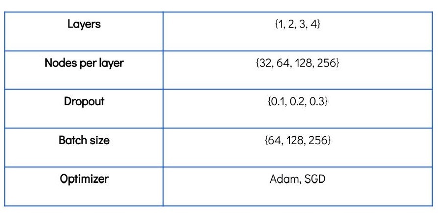
The table below shows the set of hyperparameters used in the training and optimization. Since there was no built-in hyperparameter search option in pycox package, this parameters were derived manually.
The final choice (lr = 0.001, batch_size = 128, number_nodes = 256) was based on the smallest loss value (it equals -7.2678223). Comparing to the standard CoxPH (where the loss was $\approx$ -14.1) it is a significant improvement.
5.2 DeepHit
The model called “DeepHit” was introduced in a paper by Changhee Lee, William R. Zame, Jinsung Yoon, Mihaela van der Schaar in April 2018. It describes a deep learning approach to survival analysis implemented in a tensor flow environment.
DeepHit is a deep neural network that learns the distribution of survival times directly. This means that this model does not do any assumptions about an underlying stochastic process, so both the parameters of the model as well as the form of the stochastic process depends on the covariates of the specific dataset used for survival analysis. [18]
The model basically contains two parts, a shared sub-network and a family of cause-specific sub-networks. Due to this architecture a great advantage of DeepHit is that it easily can be used for survival datasets with one single risk but also with multiple competing risks.
The dataset used so far describes one single risk, the risk of default. Customers that did not experience the event of interest are censored. The reasons for censorship can either be that the event of interest was not experienced or another event happened that also led to the end of observation, but is not the event of interest for survival analysis.
The original dataset has information about a second risk, the early repayment, also called payoff. For prior use the dataset was preprocessed in a way that customers with an early repayment were also labelled censored, because the only event of interest was the event of default. If the second risk also becomes the focus of attention in terms of survival analysis a second label for payoff (payoff = 2) can be introduced in the event column of the dataset. Therefore a competing risk is an event whose occurrence precludes the occurrence of the primary event of interest. [19]

The graph below shows the distribution of the target variable time to event within the dataset for competing risks. In total more customers experience the event of payoff than face the event of default or become censored. Throughout the observation time most of the customers who pay off early, repay their mortgage within the first year. The proportion of the customers who default is also high within the first year. The amount of payoffs as well as defaults per month decreases after the first year. Most of the censored customers are censored sometime after 2.5 years besides a peak of censored customers at the ninth month.

To also handle competing risks DeepHit provides a flexible multi-task learning architecture.
Multi-task learning was originally inspired by human learning activities. People often apply the knowledge learned from previous tasks to help learn a new task. For example, for a person who learns to ride the bicycle and unicycle together, the experience in learning to ride a bicycle can be utilized in riding a unicycle and vice versa. Similar to human learning, it is useful for multiple learning tasks to be learned jointly since the knowledge contained in a task can be leveraged by other tasks.
In the context of deep learning models, multiple models could be trained, each model only learning one task (a). If this multiple tasks are related to each other, a multi-task learning model can be used with the aim to improve the learning of a model by using the knowledge achieved throughout the learning of related tasks in parallel (b). [20]
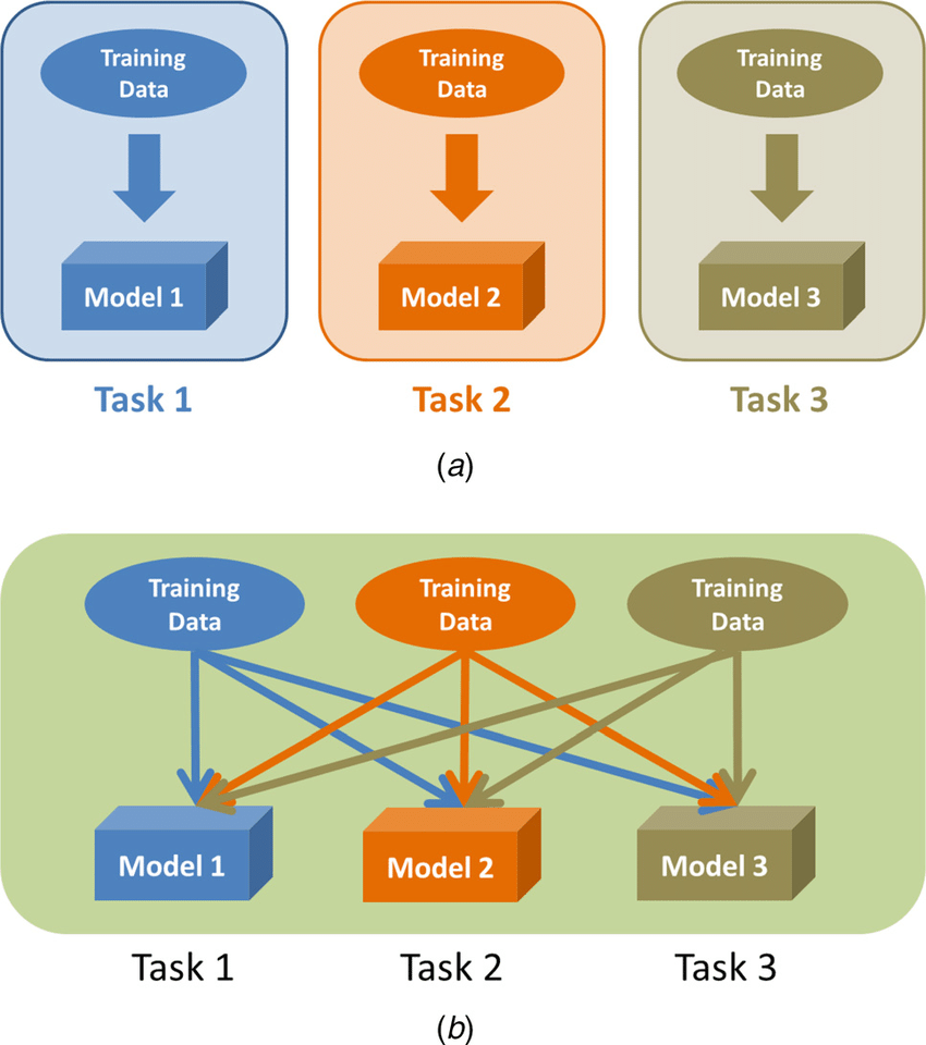 (Source: [20a])
Multi-task learning is similar to transfer learning but has some significant differences. Transfer learning models use several source tasks in order to improve the performance on the target task. Multi-task learning models treat all tasks equally, there is no task importance hierarchy. There is no attention focus on one specific task. The goal of multi-task learning models is to improve the performance of all tasks.
The most commonly used approach to multi-task learning in neural networks is called hard parameter sharing. The general architecture of such a multi-task learning model describes two main parts. The first part is a shared sub-network, where the model learns the common representation of the related tasks. The model then splits into task-specific sub-networks in order to learn the non-common parts of the representation. The number of task-specific sub-networks is equal to the number of related tasks the model is trained on. For the sake of completeness another approach to multi-task learning is soft parameter sharing that describes an architecture where each task has its own model with its own parameters. To encourage the parameters to become similar, regularisation techniques are applied between the parameters of the task-specific models. Since DeepHit provides an architecture of hard parameter sharing, the approach of soft parameter sharing will be neglected in further explanations.
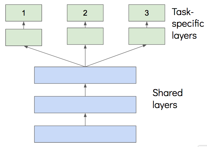 (Source: [20b])
To train a multi-task learning model just as many loss functions as tasks are required. The model is then trained by backpropagation. The fact that the task-specific sub-networks share common hidden layers, allows comprehensive learning. Through the shared hidden layers, features that are developed in the hidden layers of one task can also be used by other tasks. Multi-task learning enables features to be developed to support several tasks which would not be possible if multiple singe-task learning models would be trained on the related tasks in isolation. Also some hidden units can specialise on one task, providing information that are not important for the other tasks. By keeping the weights to these hidden units small gives these tasks the opportunity to ignore these hidden units. [21]
With multi-task learning a model can increase its performance due to several reasons. By using the data of multiple related tasks, multi-task learning increases the sample size that is used to train the model which is a kind of implicit data augmentation. The network sees more labels, even though these labels are not the labels from the same task but highly related tasks. A model that learns different similar tasks simultaneously is able to learn a more general representation that captures all of the tasks.
Moreover by learning multiple tasks together the network has to focus on important information rather than task-specific noise. The other tasks provide additional evidence for the relevance or irrelevance of the features and help to attract the network´s attention to focus on the important features.
Some tasks are harder to learn even by themselves. A model can benefit from learning the hard task combined with an easier related task. Multi-task learning allows the model to eavesdrop, learn the hard task through the simple related task, and therefore learn the hard task easier and faster than learning the hard task in isolation.
In addition different related tasks can treat each other as a form of regularisation term since the model has to learn a general representation of all tasks. Learning the tasks in a single-task learning approach would bear the risk of overfitting on one task. [22]
(Source: [22a])
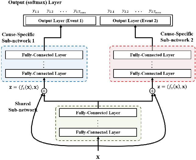
The architecture of the DeepHit model is similar to the conventional multi-task learning architecture of hard parameter sharing, but has two main differences. DeepHit provides a residual connection between the original covariates and the input of the cause-specific sub-networks. This means that the input of the cause-specific sub-networks is not only the output of the preceded shared sub-network but also the original covariates. These additional input allows the cause-specific sub-network to better learn the non-common representation of the multiple causes.
The other difference refers to the final output of the model. DeepHit uses one single softmax output layer so that the model can learn the joint distribution of the competing events instead of their marginal distribution. Thus the output of the DeepHit model is a vector $y$ for every subject in the dataset giving the probabilities that the subject with covariates $x$ will experience the event $k$ for every timestamp $t$ within the observation time. The probabilities of one subject sum up to 1.

The visualisation of the DeepHit model shows the architecture for a survival dataset of two competing risks. This architecture can easily be adjusted to more or less competing risks by adding or removing cause-specific sub-networks. The architecture of the DeepHit model depends on the number of risks.
To implement the model the DeepHit repository has to be cloned to create a local copy on the computer.
DeepHit also needs the characteristic survival analysis input setting containing the event labels, the durations as well as the covariates. A function is provided that either applies standardisation or normalization of the data. For this analysis standardisation was applied on the data.
The variable num_Category describes the dimension of the time horizon of interest and is needed in order to calculate the output dimension of the output layer of the model. num_Event gives the number of events excluding the case of censoring, since censoring is not an event of interest. This number defines the architecture of the model, it specifies the number of cause-specific sub-networks and is also needed to calculate the dimension of the output layer, which is the multiplication of num_Category and num_Event. The input dimension is defined by the number of covariates used to feed the network.
The hyperparameters of DeepHit can be tuned by running random search using cross-validation. The function get_random_hyperparameters randomly takes values for parameters out of a manually predefined range for those parameters. Possible candidates for parameter tuning can be:
- Batch size
- Number of layers for the shared sub-network
- Number of layers for the cause-specific sub-network
- Number of nodes for the shared sub-network
- Number of nodes for the cause-specific sub-network
- Learning rate
- Dropout
- Activation function
The chosen parameters are forwarded to the function get_valid_performance along with the event labels, durations and covariates (summarized in DATA) as well as the masks for the loss calculations (summarized in MASK). This function takes the forwarded parameters to build a DeepHit model corresponding to the number of events of interest as well as the number of layers and nodes for the sub-networks. The dataset is then spilt into training, validation and test sets in order to start training the model on the training set using the chosen parameters. The training is done with mini batches of the training set over 50.000 iterations. Every 1000 iteration a prediction is done on the validation set and the best model is saved to the specified file path. The evaluation of the models is based on the concordance index. The best result (= highest concordance index) is returned if there is no improvement for the next 6000 iterations (early stopping). The concordance index is a measure for survival analyis models and is explained in detail in the evaluation part of this blog post.
DeepHit is build with Xavier initialisation and dropout for all the layers and is trained by back propagation via the Adam optimizer. To train a survival analysis model like DeepHit a loss function has to be minimised that is especially designed to handle censored data.
The loss function of the DeepHit model is the sum of two terms.
$L_{1}$ is the log-likelihood of the joint distribution of the first hitting time and event. This function is modified in a way that it captures censored data and considers competing risks if necessary. The log-likelihood function also consists out of two terms. The first term captures the event and the time, the event occurred, for the uncensored customers. The second term captures the time of censoring for the censored customers giving the information that the customer did not default up to that time.
$L_{2}$ is a combination of cause-specific ranking loss functions since DeepHit is a multi-task learning model and therefore needs cause-specific loss functions for training. The ranking loss function incorporates the ** estimated cumulative incidence function ** calculated at the time the specific event occurred. The formula of the cumulative incidence function (CIF) is as follows:
This function expresses the probability that a particular event k occurs on or before time t conditional on covariates x. To get the estimated CIF, the sum of the probabilities from the first observation time to the time, the event k occurred, is computed.
The cause-specific ranking loss function adapts the idea of concordance. A customer that experienced the event k on a specific time t should have a higher probability than a customer that will experience the event sometime after this specific time t. The ranking loss function therefore compares pairs of customers that experienced the same event of interest and penalizes an incorrect ordering of pairs.
After the training process the saved optimised hyperparameters as well as the corresponding trained model can be used for the final prediction on the test dataset.
6. Evaluation
6.1 Concordance index
For the evaluation of survival analysis models the performance measures need to take censored data into account. The most common evaluation metric in survival analysis is the concordance index (c-index). It shows the model’s ability to correctly provide a reliable ranking of the survival times based on the individual risk scores. The idea behind concordance is that a subject that dies at time t should have a higher risk at time t than a subject who survives beyond time t.
- The concordance index expresses the proportion of concordant pairs in a dataset, thus estimates the probability that, for a random pair of individuals, the predicted survival times of the two individuals have the same ordering as their true survival times. A concordance index of 1 represents a model with perfect prediction, an index of 0.5 is equal to random prediction. [23]
For a better understanding of this definition the concordance index is calculated on some simple example predictions. The following table shows the true default times of four theoretical customers along with default time predictions of three different models.
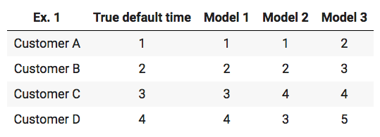
To calculate the concordance index the number of concordant pairs has to be divided by the number of possible ones. By having four customers the following pairs are possible: (A,B) , (A,C) , (A,D) , (B,C) , (B,D) , (C,D). The total number of possible pairs is 6.
- Model 1 predicts that A defaults before B, and the true default time confirms that A defaults before B. The pair (A,B) is a concordant pair. This comparison needs to be done for every possible pair. For the prediction of Model 1 all possible pairs are concordant, which results in an Concordance index of 1 - perfect prediction.
- For the prediction of Model 2 there are five concordant pairs, but for the pair (C,D) the model predicts that D defaults before C, whereas the true default times show that C defaults before D. With this the concordance index is 0.83 (5/6).
- The concordance index of Model 3 is also equal to 1, since the model predicts the correct order of the possible pairs even though the actual default times are not right in isolation.
The next example shows the computation of the concordance index in case of right-censoring:
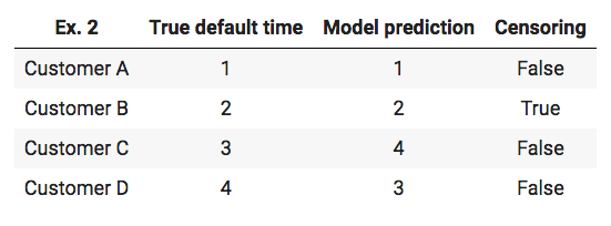
The first step is to figure the number of possible pairs. The default times of customer A can be compared to the default times of the other customers. The customer B is censored, which means that the only information given is the fact that customer B did not default up to time 2, but there is no information if customer B will default and if so, when the customer will experience the event of default. Therefore a comparison between customer B and C as well as customer B and D is impossible because these customers defaulted after customer B was censored. The comparison between customers C and D is possible since both customers are not censored. In total there are four possible pairs: (A,B) , (A,C) , (A,D), (C,D) The second step is to check if these possible pairs are concordant. The first three pairs are concordant, the pair (C,D) is discordant. The result is a concordance index of 0.75 (3/4). [24]
The dataset used for the blog post features the case of right-censoring but the reason for censoring is that these customers are still in the phase of repaying and their loans have not matured yet. Therefore the time of censoring is equal to the last observation time. Due to this the case that some customer default after a customer was censored is not possible. The example of the concordance index in case of right-censoring is shown for the sake of completeness since other survival datasets can have this case. A medical dataset for example can have data about patients with a heart disease. If a patient dies due to different reasons than a heart disease this patient would be censored. This can happen during the observation time and other patients can die due to a heart disease at a later time.
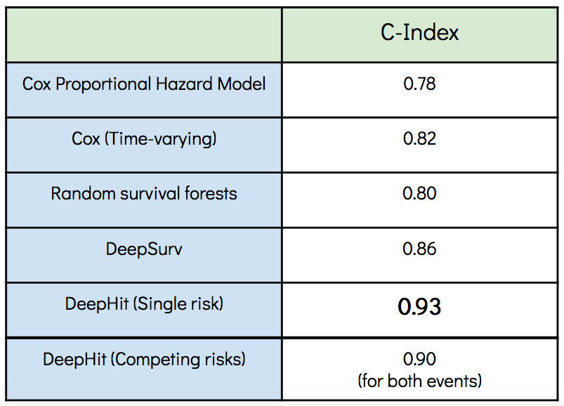
The table shows the concordance indices of the models trained with the mortgage dataset. The benchmark models, CoxPH and Random survival forests, start with a convenient performance but are outperformed by the deep learning models whereas the DeepHit model achieved the highest concordance index.
After evaluating the performance of the models we have a look into the output of the two best performing models, DeepSurv and DeepHit.
6.2 DeepSurv - Survival curves
As we have already learned before in part 4.1 about Kaplan-Meier estimator, survival curve represents a statistical graphical interpetation of the survival behaviour of subjects (i.e. mortgage borrowers) in the form of a graph showing percentage surviving vs time. This allows to examine and compare estimated survival times for each individual (except Kaplan-Meier model) and define global patterns in data (in example, sharp lines which go close to 0% propability may have certain explaination).
The graph below represents the estimated survival lifetimes for 15 individual mortgage borrowers from the test dataset using the output of the DeepSurv model. According to the graph, for a significant amount of customers the predicted survival times decrease within the first two years. For instance, for the customer with ID 5 the survival function shows that after 15 months he has a probability of roughly 50% to survive beyond 15 months. Whereas the survival function of customer with ID 9 at the same point in time shows that he has only 25% chance to survive beyond this time.
By the end of our study there is a certain flatten part at $t \approx 42$ months for some number of customers. The possible reason behind this can be due to provided individual “treatments” by the bank e.g. in order to reduce the maturity time.

6.3 DeepHit - Hazard graphs
The output of the DeepHit model is a vector for every customer giving the probabilities of the customer experiencing the event of interest for every point in time. The evaluation time is 72 months. Therefore the output gives 72 probabilities for every customer experiencing the event of default (single risk). It is the joint distribution of the first hitting time and event, hence the sum of the probabilities of a customer is equal to 1. The following graph displays the visualisation of the output of every customer included in the test set (10.000 customers).

The graph shows that in the beginning there seems to be a higher risk of default which is decreasing within the first two years which also matches to the predicted survival curves of the DeepSurv model. Throughout the evaluation time there are several probability increases for individual customers. There is a higher risk of default after the second and third year as well as within the period of the fifth and sixth year of credit time. Unfortunately it is not possible to compare these specific times to actual events in the past to derive any reasons for these peaks since the periods of the mortgage dataset used for this analysis are deidentified. Thus it cannot be retraced when the data for this dataset was collected.
To get a closer look at the individual hazard graphs in order to compare the prediction of the model to the true default times the hazard graphs of a selection of six customers is plotted.


For the most part the hazard graphs of these customers show that within the first year the probability of default is higher and mostly decreasing within the second year.
- Hazard graph 1 also represents this trend. Throughout the rest of the evaluation time the probability values decrease and range between 0.5% and 2%. In the dataset the customer was censored after 26 months. With regard to the predicted hazard ratio if the customer “survives” beyond the first year he probably does not experience the event of default afterwards.
- Hazard graph 2 starts with a high default probability after 3 months. With respect to the actual values, the customer defaulted after 3 months, the model could make a precise prediction.
- Hazard graph 3 shows the highest values within the time of 10 and 13 months after initial recognition of the mortgage which represents the actual values of the customer defaulting after 13 months.
- Hazard graph 4 differs from the other graphs since it starts with low risk of default period. The probability is not decreasing until the start of the sixth year of credit time except a little increase at the end of the second year. The model predicts that if the customer will experience the event of default it will be sometime after the fifth year of credit time. The customer was censored after 39 months, he is still repaying his mortgage rates and has not experienced the event yet.
- The customers of Hazard graph 5 and 6 were censored after a short time interval. They both have an increased risk of default within the first year. For customer 5 the second and third year is a low risk period, followed by years of higher risk of default. Hazard graph 6 shows a decrease in hazard after the second year but like the Hazard Rate 1 and 3 the probabilities vary between low values until the end of evaluation time.
In case of two competing risks the output of DeepHit is a vector of length 144 for every customer. This length comes from 72 probabilities of experiencing event 1 (default) and 72 probabilities of experiencing event 2 (payoff). The vector gives the joint probability distribution of both events, so the sum of a vector of one customer is equal to 1.
To get an overview of the predictions the output of every customer per event is visualised. When comparing the graphs the different ranges of the probability of risk have to be noted. The first graph shows the hazard ratios of the customer experiencing the event of default. In the beginning the risk of default is higher but decreases within the first two years reaching a low risk period within the years three and four. After that period the probability to default increases locally and for some individual customers the model predicts the highest risk of default after 5 years which is probably a result due to the censored data.
The risk of payoff is compared to the default risk higher in the beginning, since in total more customers experience the event of payoff than the event of default. It is slightly decreasing throughout the first 4.5 years, for some customers the event of payoff is pretty likely within the fifth year.

Looking at selected individual hazard graphs plotting the joint distribution of both events per customer to compare the predictions with the true event times of the selected customers.

- Hazard Graph 1 gives a higher probability of experiencing default than payoff. Moreover the model predicts the default to be at the end of first year, which matches the true default time of the customer experiencing the event of default after 13 months.
- The Hazard Graph 2 starts with a low risk period of more than two years regarding both events. After 2.5 years the risk of early repayment is increasing but after four years of credit time the model also predicts a strong increased hazard in default. In total the model predicts a slightly higher risk of payoff. The customer was censored after 39 months, which corresponds to the long period of low risk to experience one of these events, but with regard to this customer the model is not able to make a strong prediction to either default or payoff.
- The Hazard Graph 3 shows a high risk of payoff right in the beginning. The prediction represents the customers true event time of experiencing the event of payoff after 1 months.
- Hazard Graph 4 is similar to the third graph and also leads to a good prediction of payoff after 4 months which matches the actual values of the customer. The graph shows a sudden increase in payoff risk around 4.5 years that again decreases to a zero risk afterwards which is probably a result of the pattern the model learned, but looks more like an unrealistic outlier.
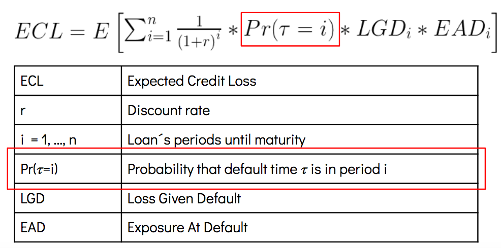
Mostly the DeepHit models for single as well as for competing risks can already make great predictions on the test dataset. With regard to the initial introduced business case, the predicted probability values of each customer can be used in order to calculate the expected credit loss to set up the provisions as a counterbalance to the recognised values of the loans. The formula of the expected credit loss is:
(Source: [27])
The output of survival analysis provides the probability values to fill the part of the formula in the above red box. The more precise the prediction of the survival analysis models the more exact calculations of the expected credit losses is possible which has an impact on the bank’s income statement.
7. Conclusion
We hope that our blog post gives everyone a clear overview of survival analysis and probably inspires to use it in further academic or professional work. The standard survival statistics, such as the Cox proportional hazards model, already allows to gain a meaningful insight from data without any sophisticated implementation of the model.
The advanced extension of survival analysis models using machine learning practices gives more methodological freedom. With proper hyperparameter tuning process it is possible to achieve more precise predictions of the time-to-event target variable.
The format of the dataset is exceptionally important. In order to apply survival analysis techinques, the data has to meet the requirements of the characteristic survival analysis data points: event, duration and valuable features.
The implementation of more complex survival analysis models in Python is still in development. With increasing popularity of this methods in different industries we hope that it is just a question of time that the variety of functions within the survival analysis packages will rise.
Thanks for reading our blogpost and surviving it :)
8. References
[1] IFRS 9 Financial Instruments - https://www.ifrs.org/issued-standards/list-of-standards/ifrs-9-financial-instruments/#about (accessed: 29.01.2020)
[2] Ernst & Young (December 2014): Impairment of financial instruments under IFRS 9 - https://www.ey.com/Publication/vwLUAssets/Applying_IFRS:_Impairment_of_financial_instruments_under_IFRS_9/$FILE/Apply-FI-Dec2014.pdf
[3] Bank for International Settlements (December 2017): IFRS 9 and expected loss provisioning - Executive Summary - https://www.bis.org/fsi/fsisummaries/ifrs9.pdf
[4] Liberato Camilleri (March 2019): History of survival snalysis - https://timesofmalta.com/articles/view/history-of-survival-analysis.705424
[5] Sucharith Thoutam (July 2016): A brief introduction to survival analysis
[6] Taimur Zahid (March 2019): Survival Analysis - Part A - https://towardsdatascience.com/survival-analysis-part-a-70213df21c2e
[7] Lore Dirick, Gerda Claeskens, Bart Baesens (2016): Time to default in credit scoring using survival analysis: a benchmark study
[8] lifelines - Introduction to survival analysis - https://lifelines.readthedocs.io/en/latest/Survival%20Analysis%20intro.html
[9] Nidhi Dwivedi, Sandeep Sachdeva (2016): Survival analysis: A brief note - https://lifelines.readthedocs.io/en/latest/Survival%20Analysis%20intro.html
[9a] https://www.slideshare.net/zhe1/kaplan-meier-survival-curves-and-the-logrank-test
[10] Maria Stepanova, Lyn Thomas (2000): Survival analysis methods for personal loan data
[10a] https://www.statisticshowto.datasciencecentral.com/hazard-function/
[11] Hazard Function: Simple Definition - https://www.statisticshowto.datasciencecentral.com/hazard-function/ (accessed 29.01.2020)
[12] Jared L. Katzman, Uri Shaham, Alexander Cloninger, Jonathan Bates, Tingting Jiang, and Yuval Kluger (2018): DeepSurv: personalized treatment recommender system using a Cox proportional hazards deep neural network - https://arxiv.org/abs/1606.00931
[13] Hemant Ishwaran, Udaya B. Kogalur, Eugene H. Blackstone and Michael S. Lauer (2008): Random Survival Forests - https://arxiv.org/pdf/0811.1645.pdf
[14] ‘scikit-survival’ package - https://scikit-survival.readthedocs.io/en/latest/
[15] Time-to-event Analysis - https://www.mailman.columbia.edu/research/population-health-methods/time-event-data-analysis
[16] Travers Ching,Xun Zhu,Lana X. Garmire (2018): Cox-nnet: An artificial neural network method for prognosis prediction of high-throughput omics data - https://journals.plos.org/ploscompbiol/article?id=10.1371/journal.pcbi.1006076
[17] Eleonora Giunchiglia, Anton Nemchenko, and Mihaela van der Schaar (2018): RNN-SURV: A Deep Recurrent Model for Survival Analysis - http://medianetlab.ee.ucla.edu/papers/RNN_SURV.pdf
[18] Changhee Lee, William R. Zame, Jinsung Yoon, Mihaela van der Schaar (April 2018): DeepHit: A Deep Learning Approach to Survival Analysis with Competing Risks
[19] Peter C. Austin, Douglas S. Lee, Jason P. Fine (February 2016): Introduction to the Analysis of Survival Data in the Presence of Competing Risks - https://www.ahajournals.org/doi/10.1161/CIRCULATIONAHA.115.017719
[20] Yu Zhang, Qiang Yang (2018): A survey on Multi-Task Learning
[20b] https://ruder.io/multi-task/index.html#hardparametersharing
[21] Rich Caruana (1997): Multitask Learning
[22] Sebastian Rude (October 2017): An Overview of Multi-Task Learning in Deep Neural Networks
[23] PySurvival Introduction, Performance metrics, C-index - https://square.github.io/pysurvival/metrics/c_index.html#introduction (accessed 04.02.2020)
[24] Alonso Silva Allende (October 2019): Concordance Index as an Evaluation Metric - https://medium.com/analytics-vidhya/concordance-index-72298c11eac7 (accessed 04.02.2020)
[25] David Faraggi Richard Simon (1995): A neural network model for survival data - https://onlinelibrary.wiley.com/doi/abs/10.1002/sim.4780140108
[26] WTTE-RNN - Less hacky churn prediction - https://ragulpr.github.io/2016/12/22/WTTE-RNN-Hackless-churn-modeling/
[27] Bernd Engelmann (April 2018) - Calculating Lifetime Expected Loss for IFRS 9: Which Formula is Correct?