By Seminar Information Systems (WS19/20) | February 7, 2020
Anti Social Online Behaviour Detection with BERT
Comparing Bidirectional Encoder Representations from Transformers (BERT) with DistilBERT and Bidirectional Gated Recurrent Unit (BGRU)
R. Evtimov - evtimovr@hu-berlin.de
M. Falli - fallimar@hu-berlin.de
A. Maiwald - maiwalam@hu-berlin.de
Introduction
Motivation
In 2018, a research paper by Devlin et, al. titled “BERT: Pre-training of Deep Bidirectional Transformers for Language Understanding” took the machine learning world by storm. Pre-trained on massive amounts of text, BERT, or Bidirectional Encoder Representations from Transformers, presented a new type of natural language model. Making use of attention and the transformer architecture, BERT achieved state-of-the-art results at the time of publishing, thus revolutionizing the field. The techniques used to build BERT have proved to be broadly applicable and have since launched a number of other similar models in various flavors and variations, e.g. RoBERTa [8.] and AlBERT [7.].
![BERT broke the record on the SQuAD challenge. From: [Google Research]](/blog/img/seminar/bert/bert_leader_1.png)
BERT broke the record on the SQuAD challenge. From: [Google Research]
![BERT also broke the record in multiple other benchmark challenges. From: [Google Research]](/blog/img/seminar/bert/bert_leader_2.png)
BERT also broke the record in multiple other benchmark challenges. From: [Google Research]
Our goal with this blog post is to describe the theory behind the model, give insight into the Transformer architecture that makes it possible and put it to the test through a practical implementation. In order to make it easier to follow, and also help you construct your own model for a different task, the blog post is going to be accompanied by code snippets. In the last part of the post, we will examine the model’s performance and draw the concluding remarks.
Dataset
Although BERT can be used for a number of different classification tasks (e.g. sentence pair, multi-label classification), we are going to conclude a binary classification. For our task, we chose the Toxic Comment dataset from Kaggle. It consists of 159 571 Wikipedia comments, which have been manually labeled for their toxic behavior by real human raters. The comments are classified by six types of toxicity: toxic, severe_toxic, obscene, threat, insult and identity_hate. A “1” signifies that the label is true, and “0” that it is false. For the binary classification, we decided to combine all labels into one named “malicious”. The data set is imbalanced, as there are around 10% malicious and 90% non-malicious comments. The sentences were also cleaned and prepared, which we will examine more in the code.
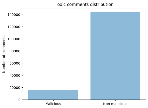
The dataset is very unbalanced.
The original dataset is available to download here: https://www.kaggle.com/c/jigsaw-toxic-comment-classification-challenge/data
Past Developments
“Drop your RNN and LSTM, they are no good!” [2.]
To better understand and grasp the importance of the methods we used for this assignment and mainly the Transformer architecture, let’s first have a brief overview of what led to these developments, and why they are deemed to be a breakthrough in NLP models.
Recurrent neural networks (RNNs) are a class of artificial neural networks that are good at modeling sequence data and processing it for predictions. They have a loop which allows for information to be transferred more easily from one particular step and the next. This information from previous inputs is the so-called hidden state.
![Recurrent neural network. From: [21.]](/blog/img/seminar/bert/rnn_loop.png)
Recurrent neural network. From: [21.]
However, RNNs have an issue known as short-term memory. Short-term memory is caused by the vanishing gradient problem. As the RNN processes more steps, it has trouble keeping information from prior ones. For example, let’s say we have the sentence “BERT is my best friend and I love him” which is fed through an RNN. The first step is to feed “BERT” into the network. The RNN encodes it and produces an output. Next, the word “is” and the hidden state from the previous step are processed. Now, the RNN has information on both words “BERT” and “is”. In this way, the process is repeated until the end of the sentence. However, when reaching the last time step, the information about the first two words is almost non-existent. Therefore, because of vanishing gradients, RNNs have trouble learning the long-range dependencies across different time steps.
To mitigate short-term memory, Long Short-Term Memory networks, or LSTMs were developed. The key improvement over RNNs is the cell state or the memory part of the network. It goes straight through the entire network, which allows for information to flow easily with minor adjustments made through “gates”. Gates are different tensor operations that can learn what information to add or to remove from the hidden state. This means that LSTMs are able to mitigate some of the vanishing gradient problem - an improvement over RNNs. However, the problem is only partially solved. There is still a sequential path from older past cells to the current one. LSTMs can, therefore, learn a lot more long-term information, but they have trouble remembering sequences of thousands or more.
![Long Short Term Memory network. From: [21.]](/blog/img/seminar/bert/lstm.png)
Long Short Term Memory network. From: [21.]
The next evolution in trying to solve this problem was in the form of convolutions in CNNs, or Convolutional Neural Networks. RNNs and LSTMs work great for text but convolutions can do it better and faster. And, as any part of a sentence can influence the semantics of a word, we want our network to see a much larger part of the input at once. For example, DeepMind’s WaveNet is a fully convolutional neural network, where the convolutional layers allow it to grow exponentially and thus cover a large number of time steps [10.]. This means that CNNs are not linear like LSTMs. However, they still seem to be referencing words very much by position, when referencing by content would be more beneficial.
Transformer
At the end of 2017 something new came out that completely changed the landscape in the NLP field. This was the attention algorithm. It was first introduced by the Google Brain team with the paper “Attention is all you need” (Vaswani et al., 2017) emphasizing the fact that their model does not use recurrent neural networks at all. [1.] [16.] Attention had already been a known idea used in LSTMs, but this was the first time it completely took the place of the recurrence. In the following paragraphs, the main idea of “The Transformer” model will be explained.
“The Transformer” is a seq2seq model created for machine translation. The task it is targeting plays an important role in the structure: Encoder-Decoder architecture ending with a softmax “plain vanilla” neural network. [21.]
The innovation of the paper consists of the attention mechanism. In order to understand the current developments in the NLP field, it is important to have a deep understanding of the concept and the way it functions in practice.
![Encoder Decoder Structure. Adapted from [1.]](/blog/img/seminar/bert/encoder_decoder.jpg)
Encoder Decoder Structure. Adapted from [1.]
Purpose of Attention
As already mentioned in the previous part scientists were trying to find a solution for the short-term memory to be able to better represent the human language.
How could the model learn which words and their meaning are connected to each other and which stay in one sentence, but don’t have a strong semantic connection? The paper introduces a way for the model to calculate the importance of any word and help it pay “attention” only to the words that are more important.
Every NLP model works with word embeddings (vector representation of the word). We are going to track the whole movement and change of those embeddings to understand how attention is calculated.
As illustrated in the following picture, from the initial sequence for every word we create a word embedding and multiply it to 3 different matrices. As a result, we get three different vectors - Query, Key and Value. They are different representations of the same initial word embedding.
The whole idea of “attention” is to calculate the dot product of Q of one token(word) and K of another. Doing this for the Q of one word and the K of all other words in the sequence, we calculate which ones are more important than others. This would mean the words that lead to a higher dot product have greater importance for the word we are calculating this for. After we have calculated this value for every pair, we take all of them and using a softmax function calculate weights corresponding to the importance of every word for the current one. The model then multiplies the weights to the V matrix of each word, sums them up and creates a new vector representation of the initial word.
To summarize: the attention mechanism takes an embedding, calculates 3 different matrices, then based on two of them calculates the importance of every word for the other, then creates a weight that represents this importance and comes out with a new embedding representing this position in the sequence.
One should be able to understand where those three matrices come from. In the beginning, they are randomly initiated and learned during the training process. [11.]
![Calculation of Attention. Adapted from [1.]](/blog/img/seminar/bert/mamu_2.png)
Calculation of Attention. Adapted from [1.]
Multi-head Attention
After the initial idea and mechanism of attention it is important to distinguish that this is not what exactly happens in the original model. What the original model uses, is called “multi-head attention”. Multi-head attention basically means that the process explained in the previous paragraph is repeated 8 different times with different randomly initiated matrices.
Logically at the end of the process, we have done the same thing with 8 different matrices. As input in the next layer is again a vector similar to the initial one in size. To do this we have to reduce the dimensionality of the matrix that resulted from those 8 different “attention heads”. For this purpose the model learns an additional weight matrix, that shows which attention head is more important for the meaning of the words and which not. Again, this matrix is randomly initialized and are being calculated during the training process. [9.]
The following graph gives a better overview of how the attention heads calculate their values and how the input for the next layer is “produced”:
[Picture: Concatenation of heads and producing output of layers]
Concatenation of different attention heads. From: [1.]![Concatenation of different attention heads. From: [1.]](/blog/img/seminar/bert/transformer_concat.jpeg)
Naturally, a person would want to be able to evaluate if attention makes sense, we can have a look at why each attention head produces as a result. For a human, a logical means to do this is if after looking at the weights every attention head calculates a different, clear type of connection for a word with the rest of the words in a sequence. As we know, it is often extremely hard for a human to understand what a machine learning model is doing to produce its result. It is usually not easy to follow how the flow of information ends up in a correct prediction. This case is no exception: the following graph illustrates the different attention heads and the coefficients they come up with to represent the link between different words. Every color represents one attention head and in every layer, there are 8 different attention heads. Only for a small amount of them, we are able to really understand why they are connected in a certain way.
For example, certain heads consider mainly the link to the first word in the sequence which doesn’t necessarily make sense for a human observing the results.
Types of Attention
After talking about how the mechanism is calculated in the Encoder, a correct explanation has to distinguish between different types of attention within the original model. What was explained until now was the Encoder Self-attention, but this is only one of the ways it is being calculated: We have a couple of other ways: “Encoder-Decoder attention” and “Masked Decoder Self-Attention”.
Encoder-Decoder attention: the task of the model is machine translation. Of course, the decoder has to produce a translated sequence and the prediction is based on the attention calculated in the encoder. This happens in this part of the model where the Decoder takes certain information from the Encoder and produces a prediction about the next word in the sequence. This is to be seen also in the following figure. [6.]
Masked Decoder Self-Attention: In order to figure out what to predict as next word, the Transformer is taking information from the Encoder and looks also at its previous prediction (the words already predicted by the Decoder) The reason this type of attention is masked is because if we want a model to predict a word we are not supposed to show it the result it has to produce. Masked means all tokens except the previous ones are isolated from the equation.
Looking at the following graph illustration of the concept could be seen. The type of attention that is obviously bidirectional is the Encoder Self-Attention. This is an essential part of the architecture of BERT.
![Three ways of attention. From: [26]](/blog/img/seminar/bert/three_attention.png)
Three ways of attention. From: [26]
Positional Encoding
There are many advantages of using Transformer instead of the popular up to this point RNN (Recurrent Neural Networks), those include:
- Simpler operations
- Better results
- Possible parallelization
However, there is an important piece of information we skip when using it: the position of the word. The order of words is crucial for understanding human language, a change of position could totally change the meaning of a sentence. A proper machine translation should be taking the word order into account. The way this is done in this model is by using positional encodings. Those are vectors representing the position of the word in a sequence (sentence). This is summed up with the initial word embedding and the model is let to learn it in the training process.
They use two functions to be calculated for each position - sine, and cosine. Using those, the authors create a unique vector for each position in the sequence. The residual connection plays an important role as with using it, the model is adjusting more easily learning the position of words and learns to distinguish the position of the word based on the sum of the initial word embedding and the positional encoding.
![Positional Encoding. From: [27.]](/blog/img/seminar/bert/pos_encoding.png)
Positional Encoding. From: [27.]
Residual connection and layer normalization
After understanding how the Encoder and Decoder layers work, it is important to note that there is another part of each layer that remains still unexplained. Namely the residual connection and layer normalization that come after every sublayer. [15.]
The residual connection is adding the initial vector to the result after each sublayer (Multi-Head attention or Feed Forward neural network). This is done to tackle the Vanishing gradient problem and retaining information about the position in adding to the output of every sublayer.
![Residual Connection. Adapted from: [28.]](/blog/img/seminar/bert/residual_connection.png)
Residual Connection. Adapted from: [28.]
Layer normalization
The layer normalization is a bit different than the often used batch normalization. Batch normalization has its limits and this is why layer normalization was introduced later. [20.] The basic intuition behind using normalization techniques is to introduce to each layer an input of similar distribution which should result in accelerating the training process. The following image explains better the differences between the two:
Summary about “The Transformer”
After clarifying the functions of the different parts of the “Transformer” model, it is needed to mention how the original model functions as a whole.
There are six encoder and six decoder layers. In each of them, there is the Multi-Head attention sublayer and the Feed-forward network, each followed by layer normalization and residual connection.
The only difference in the Decoder layer is that it includes another type of sublayer: “Encoder-Decoder attention” where the output from the Encoder is imported.
The output of all Decoders is fed into a linear layer and using a softmax function the model predicts which is the most probable next word in the sequence.
Then the whole process is repeated, taking into account also the previously predicted word.
BERT
Architecture
The architecture of the BERT model is a multi-layer bidirectional transformer encoder. It is based on the original implementation of Vaswani et al. [16].
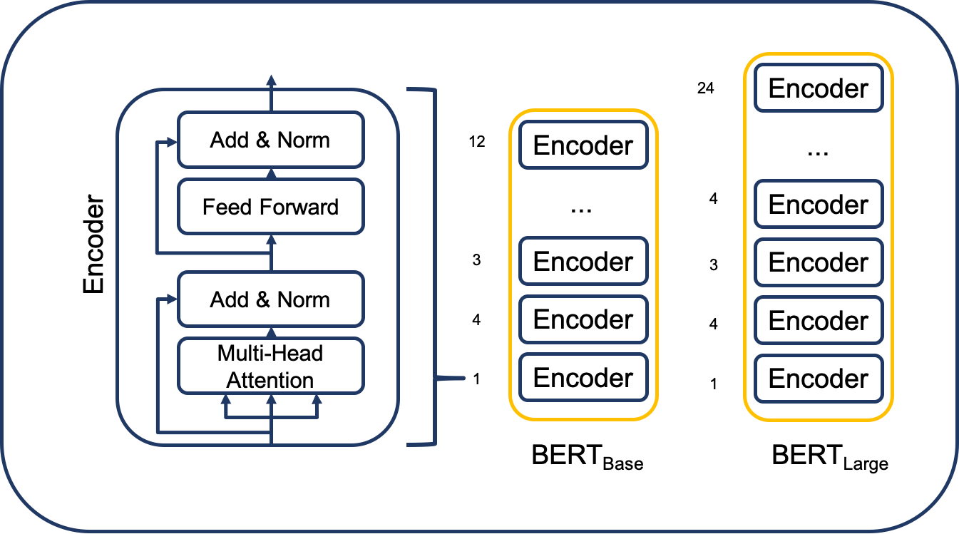
BERT Encoder Stack. Own visualization.
There are two model sizes of BERT: BERT Base and BERT large. In the following description, we denote the number of layers as L, the hidden size as H and the number of self-attention heads as A. The differences in model sizes between BERT Base and BERT Large are shown in the following table.
![Differences between BERT Base and BERT Large. Adapted from: [5.]](/blog/img/seminar/bert/bert_sizes.png)
Differences between BERT Base and BERT Large. Adapted from: [5.]
The publishers of BERT chose to develop BERT with different model sizes because they wanted to compare BERT to earlier models. Therefore they created BERT Base which has the same model size as Open AI GPT. They created a larger model to outperform the BERT Base model [3.].
Applications
In contrast to earlier pre-trained language models like OpenAi GPT or ELMo, BERT is deeply bidirectional [Google AI Blog]. This means that BERT representations are jointly trained on the left and right context in all layers, visualized in the figure below.
Another advantage of BERT is that it can be used for different approaches. BERT allows ectracting the pre-trained embeddings. These can be used in a task-specific model. This is called the feature-based approach. The main approach, however, is to fine-tune the pre-trained model on task-specific data, without making significant changes to the model. This is called the feature-based approach. The approach chosen in this blog post is the fine-tuning approach [3.].
![OpenAI GPT and ELMo are not deeply bidirectional. From: [Google AI Blog]](/blog/img/seminar/bert/other_architecture.png)
OpenAI GPT and ELMo are not deeply bidirectional. From: [Google AI Blog]
Pre-training BERT
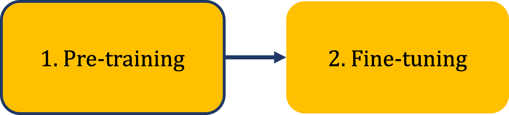
BERT strenths lies in the pretrained models. Own visualization
BERT is developed in two steps. The first one is pre-training. The data used for pre-training is a huge unlabeled data set, consisting of the English Wikipedia and BooksCorpus. The pre-training tasks are Masked Language Modeling (MLM) and Next Sentence Prediction (NSP). BERT uses a specific input format for the data to pretrain the model. This input format is described in the following part.
Input
BERT is trained with tokens. These tokens are the sum of three different embeddings of the textual data. Machine learning models cannot understand text. Textual data, therefore, needs to be transformed into numbers. BERT uses the WordPiece tokenizer for this. The WordPiece tokenizer consists of the 30.000 most commonly used words in the English language and every single letter of the alphabet. If the word, that is fed into BERT, is present in the WordPiece vocabulary, the token will be the respective number. However, if the word does not exist in the vocabulary it gets broken down into pieces until these pieces are found in the vocabulary. In the worst-case scenario a word is broken down into every single letter. To remember which tokens are pieces of a word the tokenizer uses two number signs (##).
There are three special tokens added to each sequence. A [CLS] token at the beginning, which is used for classification tasks, a [SEP] token between the first and the last part of a sequence and a [SEP] token at the end of each token. The second embeddings that BERT uses are segment embeddings. They are used to discern between the first and last part of a sequence (necessary for the pre-training tasks). The third embeddings are the positional embeddings, which simply remember the position of each word in a sequence. These three embeddings are summed up and make up the input, that is fed into BERT.
![The input for BERT consists of three embedding layers. Adapted from [3.]](/blog/img/seminar/bert/bert_input.png)
The input for BERT consists of three embedding layers. Adapted from [3.]
Tasks
Masked Language Modelling
BERT is pre-trained with two different tasks. The first one is Masked Language Modeling. Its purpose is to train for bidirectionality. In each sequence, some of the words are masked and the model has then to predict these masked words. In each sequence, 15% of the words are selected. of these selected words, 80% are exchanged with a [MASK] token. 10% of the words are exchanged with a different word and 10% are left unchanged. The aim is to bias the representation towards the actual word.
![Masked Language Modelling was used to bias to train for bidirectionality. Adapted from: [3.]](/blog/img/seminar/bert/bert_mlm.png)
Masked Language Modelling was used to bias to train for bidirectionality. Adapted from: [3.]
Next Sentence Prediction
The other task that is used for pre-training is Next Sentence Prediction. It aims to capture relationships between sentences. Given two sentences A and B, the model has to predict whether sentence B is following sentence B. This is the case 50% of the time. This task is the reason why the input tokens also comprise embeddings to discern between sequence segments.
Pretraining BERT took the authors of the paper several days. Luckily, the pre-trained BERT models are available online in different sizes. We will use BERT Base for the toxic comment classification task in the following part.
![BERT was trained with Next Sentence Prediction to capture the relationship between sentences. Adapted from: [3.]](/blog/img/seminar/bert/bert_nsp.png)
BERT was trained with Next Sentence Prediction to capture the relationship between sentences. Adapted from: [3.]
BERT for Binary Classification Task
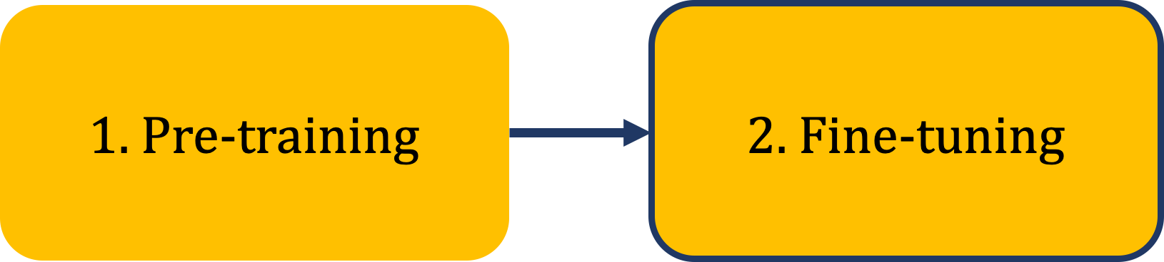
BERT can be finetuned to specific tasks. Own visualization
Evaluation Metrics
The task at hand is a binary classification task with highly unbalanced data. Hence special attention need to be paid to the metrics that are used for evaluating the performance of models. A metric that is often used for unbalanced data tasks is the area under the receiver operating characteristics (AUC ROC). However, the AUC ROC metrics have one disadvantage. Given a large number of true negatives even high changes in the number of false positives can lead to small differences in the false positive rate, that is used in the AUC ROC. Hence we report the area under the precision-recall curve (AUC PR) as well. This metric does not consider the negative in its calculation. The third metric that is reported is the F1 score [25.].
Data Preprocessing
After having explained the BERT model in detail we are now describing the necessary data preparation. In order to be able to compare results with Zinovyeva and Lessman, we followed their cleaning procedure. This entailed transforming the data to lower case, substituting negative contractions with their full version, substituting emojis with semantic equivalent, removal of stopwords, URLs, IP-addresses, usernames and non-alphanumeric characters [24.]. As the original Kaggle challenge that published the data, is now closed they supply a training and a labeled test set. However, since the labels in the test set where inconclusive, we decided to only use the training data and split it into training, validation and test sets.
As in all language models, textual data has to be tokenized before it gets fed into the model. BERT requires its input to be tokenized with the WordPiece tokenizer, which can be accessed via the BERT hub. Furthermore, the sequence length must be the same for each comment. The maximum sequence length that BERT can process is 512. As Zinovyeva and Lessman used a length of 400 we set our maximum sequence length as close as possible while avoiding out-of-memory issues [5.]. This led us to a maximum sequence length of 256 tokens. Comments that were longer than that were truncated while comments that were shorter were padded with zeros. Earlier we described that BERT uses three different embeddings summed up as tokens as input. Therefore additional segment ids and input ids were created.
![Availabe ressources restrict the max. batch size depending on the sequence length, [5.]](/blog/img/seminar/bert/oom_table.png)
Availabe ressources restrict the max. batch size depending on the sequence length, [5.]
Benchmark Model: Bidirectional Gated Recurrent Unit (BGRU)
BGRU Architecture
The aim of this blog post is to compare the performance of the sophisticated pre-trained BERT model with that of earlier and not pre-trained models. To do so we chose to compare our BERT model to the best performing BGRU of Zinoyeva and Lessmann. They used a maximum sequence length of 400 words. Because the sheer size of the BERT model limits the maximum sequence length, we could only work with a sequence length of 256. To be able to compare it with their results we modified their BGRU accordingly. The table below shows the chosen parameters as well as results.
BGRU Parameters
For the BGRU hyperparameter, we followed the previous work of Ziovyeva nd Lessmann.
BGRU Performance
The evaluation metrics showed promising results for the BGRU, especially after a very short training time.
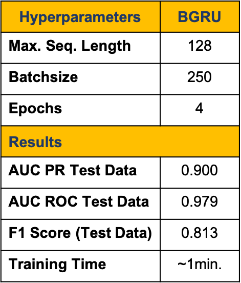
The BGRU trained quickly and yielded good results.
BERT
BERT Architecture
BERT can be implemented using different machine learning libraries. After experimenting with several libraries like HuggingFace’s Transformers and Keras we decided to use fast.ai and PyTorch as for its ease of use and the good results it yielded. PyTorch supplies pretrained BERT classes that can be downloaded easily. As we are dealing with a classification task we chose BertForSequenceClassification from PyTorch. It consists of a BERT Transformer with a sequence classification head added. Only the sequence classification head needs to be trained. It is a linear layer, that takes the last hidden state of the first character in the input sequence [pypi.org]. The loss function that we used to train our model is Binary Cross Entropy Loss.
BERT Hyperparameters
There are a number of hyperparameters that need to be set to finetune BERT. Namely: Maximum sentence length, learning rate, batch size and the number of epochs. As described earlier, the maximum sequence length has a direct impact on the maximum batch size that can be chosen. In order to find a good middle way between a batch size that is not too small, because it would lengthen the training time significantly and a sentence length that is long enough for the model to learn its meaning we chose a maxim sequence length of 256 words and a batch size of 32. As BERT is a pre-trained model, the number of training epochs can be set relatively low to 4 epochs. The learning rate we chose is the one that was recommended by the authors of BERT (3e-5).
BERT Performance
As mentioned in the introduction part, there have been a number of other models similar to BERT that have been released in the past months. One of them is Facebook’s RoBERTa [8.]. The idea behind it was to take the original BERT approach and model and make it bigger, thus helping it achieve better performance. It was trained on 160GB of text (10 times larger than BERT) and has around 15 million additional parameters compared to BERT-Base. Thanks to this it achieved new SOTA results on numerous benchmarks when it was originally published in July 2019. We wanted to compare the two in order to measure the gains of using such a larger and arguably better model. Unfortunately, we ran into computational problems when trying to implement RoBERTa for our task. Using such a large model was simply not feasible with our limited resource of hardware and cloud software. So, we looked for another comparable and, if possible, lighter model for comparison.
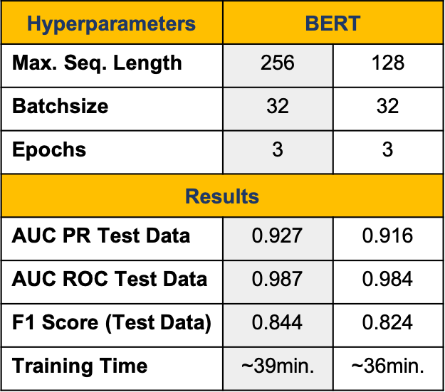
BERT outperformed the GRU regarding all three metrics but trained longer.
DistilBERT
DistilBERT [12.], developed by one of the leading ML startups Hugging Face, promises to retain around 95% of the performance while having 40% fewer parameters than BERT [13.]. The premise sounded intriguing, so we decided to use the model for our classification task and compare its performance and training time to that of BERT. We did this using simpletransformers [23.], a wrapper for Hugging Face’s transformer library. It allows to implement the model using just a few lines of code which makes it great for comparison purposes. Even though using larger batch sizes and max sequence lengths resulted in numerous resource exhaustion errors, we tried to make it as comparable as possible to our BERT approach.

DistilBERT with Simpletransformers did neither increase speed nor performance compared to BERT
Conclusion
The table below shows the results of training BERT, DistilBERT and a BGRU on the toxic comment data and testing it on unlabeled data. It shows high performance from all three models with a slight lead for DistilBERT. Additionally, BERT with two different sequence lengths was tried out, but reducing the maximum sequence length for BERT slightly decreased the results.
The main difference in the results could be observed in the auc_pr and f1_score. We choose to use the auc_pr as our main metric as the data was unbalanced and the known literature suggests this is the most suitable metric for evaluating the performance. Reducing the maximum sequence length for BERT slightly decreased the results.
There could be several reasons for the interesting results in regards to DistilBERT outperforming the others. Using DistilBERT there were no frozen layers, whereas implementing BERT without freezing layers would have been computationally expensive and wouldn’t have been possible, because of lack of resources. The BERT implementation uses only a fine-tuning process on top of the BERT-base model, making use of its powerful embeddings.
Because of the lightness of the DistilBERT model, we were able to run it for 3 epochs which took around 65 minutes. Our results confirmed the excellence of BERT and its variations, leaving the door open for further analysis of what the exact reasons for the better performance of the lighter model are.
The third model we implemented, is the BGRU. Its results also remind us that recurrence has its benefits. With a much shorter execution time, it performs nearly as good as the “Transformer” models.
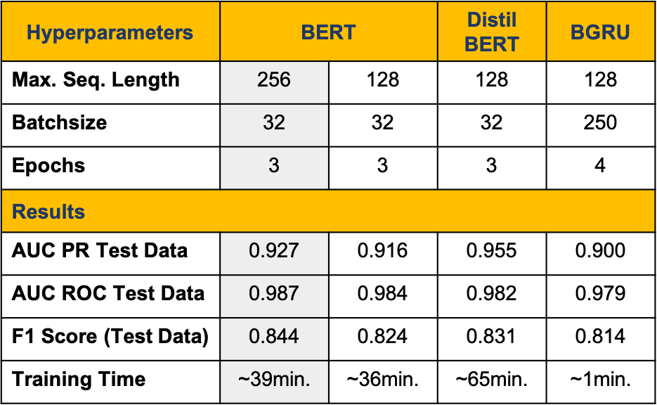
BERT outperformed DistilBERT and the BGRU
References
[1.] The Illustrated Transformer – Jay Alammar – Visualizing machine learning one concept at a time, Github. Available here: http://jalammar.github.io/illustrated-transformer/%0Ahttps://jalammar.github.io/illustrated-transformer/%0Ahttp://jalammar.github.io/illustrated-transformer/ (Accessed: 7. February 2020).
[2.] Culurciello, E. (2018) The fall of RNN / LSTM - Towards Data Science. Available here: https://towardsdatascience.com/the-fall-of-rnn-lstm-2d1594c74ce0 (Accessed: 7. February 2020).
[3.] Devlin, J. und Chang, M.-W. (2018) Google AI Blog: Open Sourcing BERT: State-of-the-Art Pre-training for Natural Language Processing, Google AI Blog. Available here: https://ai.googleblog.com/2018/11/open-sourcing-bert-state-of-art-pre.html (Accessed: 2. February 2020).
[4.] Devlin, J. u. a. (2018) „BERT: Pre-training of Deep Bidirectional Transformers for Language Understanding“.
[5.] Google/Research TensorFlow code and pre-trained models for BERT. Available here: https://github.com/google-research/bert (Accessed: 2. February 2020).
[6.] Kaiser, Ł. (1) Attention is all you need attentional neural network models – Łukasz Kaiser - YouTube. Available here: https://www.youtube.com/watch?v=rBCqOTEfxvg (Accessed: 7. February 2020).
[7.] Lan, Z. u. a. (2019) „ALBERT: A Lite BERT for Self-supervised Learning of Language Representations“.
[8.] Liu, Y. u. a. (2019) „RoBERTa: A Robustly Optimized BERT Pretraining Approach“.
[9.] Michal Chromiak The Transformer – Attention is all you need. - Michał Chromiak’s blog. Available here: https://mchromiak.github.io/articles/2017/Sep/12/Transformer-Attention-is-all-you-need/#.XFxuX89KjUI (Accessed: 7. February 2020).
[10.] Oord, A. van den u. a. (2016) „WaveNet: A Generative Model for Raw Audio“.
[11.] Rush, A. (2019) The Annotated Transformer.
[12.] Sanh,V. u. a. (2019) „DistilBERT, a distilled version of BERT: smaller, faster, cheaper and lighter“.
[13.] Sharan, S. (2019) Smaller , faster , cheaper , lighter : Introducing DistilBERT , a distilled version of BERT. Available here: https://medium.com/huggingface/distilbert-8cf3380435b5 (Accessed: 7. February 2020).
[14.] Shubham Jain (2018) An Overview of Regularization Techniques in Deep Learning (with Python code), Analytics Vidhya. Available here: https://www.analyticsvidhya.com/blog/2018/04/fundamentals-deep-learning-regularization-techniques/ (Accessed: 2. February 2020).
[15.] Tensorflow Transformer model for language understanding | TensorFlow Core. Available here: https://www.tensorflow.org/tutorials/text/transformer (Accessed: 7. February 2020).
[16.] Vaswani, A. u. a. (2017) „Attention is all you need“, in Advances in Neural Information Processing Systems. Neural information processing systems foundation.
[17.] Natural Language Processing: the age of Transformers. Available here: https://blog.scaleway.com/2019/building-a-machine-reading-comprehension-system-using-the-latest-advances-in-deep-learning-for-nlp/ (Accessed: 7. February 2020).
[18.] The Transformer for language translation. Available here: https://www.youtube.com/watch?v=KzfyftiH7R8&t=1022s (Accessed: 7. February 2020).
[19.] How Transformers Work. Available here: https://towardsdatascience.com/transformers-141e32e69591 (Accessed: 7. February 2020).
[20.] An Intuitive Explanation of Why Batch Normalization Really Works. Available here: http://mlexplained.com/2018/01/10/an-intuitive-explanation-of-why-batch-normalization-really-works-normalization-in-deep-learning-part-1/ (Accessed: 7. February 2020).
[21.] Transformer Architecture: Attention Is All You Need (2019). Available here: https://medium.com/@adityathiruvengadam/transformer-architecture-attention-is-all-you-need-aeccd9f50d09 (Accessed: 7. February 2020).
[22.] Understanding LSTM Networks – colah’s blog (2016). Available here: http://colah.github.io/posts/2015-08-Understanding-LSTMs/ (Accessed: 7. February 2020).
[23.] simpletransformers – Thilina Rajapakse (2019). Available here: https://github.com/ThilinaRajapakse/simpletransformers (Accessed: 7. February 2020).
[24.] Zinovyeva, E & Lessmann, S (2019) Antisocial Online Behavior Detection Using Deep Learning
[25.] Davis, J., Goadrich, M., 2006. The relationship between precision-recall and roc curves, in: Proceedings of the 23rd international conference on Machine learning, ACM. pp. 233–240.
[26.] Kaiser, L., Stanford NLP Available here: https://nlp.stanford.edu/seminar/details/lkaiser.pdf
[27.] Harvard NLP, 2018. Available here: https://nlp.seas.harvard.edu/2018/04/03/attention.html
[28.] Shorten, Conor, 2019. Available here: https://towardsdatascience.com/introduction-to-resnets-c0a830a288a4