By Seminar Information Systems (WS18/19) | February 9, 2019
Uncertainty in Profit Scoring (Bayesian Deep Learning)
Djordje Dotlic, Batuhan Ipekci, Julia Dullin
Contents
- Introduction
- Literature Review
- Theory
A. Bayesian Inference
B. Variational Inference
C. Monte Carlo Dropout - Data Exploration
- Results and Evaluation
Introduction
The problem of credit scoring is a very standard one in Machine Learning literature and applications. Predicting whether or not a loan applicant will go default is one of the typical examples of classification problem, and usually serves as a good ground for application and comparison of various machine learning techniques- which, over the years, became very precise in making a binary prediction. However, the credit scoring problem can be thought about as a regression problem as well. What is to be predicted here, instead of failure probability as in the classification case, is the profit rate- earnings from a loan for the lender expressed as a percentage of the amount of money loaned. The motivation for the second approach is that, even if a borrower fails to pay off the entire loan, the lender can still earn the money, and still have an interest to invest in this particular opportunity rather than some other (if profit rate is higher than in some other investment opportunity with the same risk level). The Lending Club dataset of loans from 2007-2015 (data will be properly introduced in a separate section) offers a good example of such a situation. Since it is offering a peer-to-peer landing, we can think about each loan application as an individual investment opportunity (unlike in case of bak loans where decisions are driven by some more general risk management strategies). Hence, we can treat credit scoring (and making a subsequent decision on loan granting or rejecting) as a regression problem where the information applicants are providing are used as predictors of the profit rate. The goal is to avoid “bad” loans, or, in other words, the loans that make lenders lose money.
If we are treating a loan as other securities, such as bonds, commodities, currencies, and such, we might like to assess it in a similar way regarding its risk. For tradable assets, we can follow daily price changes and formulate the expected return, volatility, skewness and kurtosis of returns distribution, which is further used for making a portfolio decision. In the case of loans, we don’t have such high-frequency data. Usually, there is some credit history, but few data points cannot lead to any reasonable assumptions about future movements. Hence, one solution would be to just use the predicted expected return or to use a classification approach.
One way around this caveat is the application of Bayesian Method in the estimation of a model. Unlike in the more traditional, deterministic, approach, the result of the prediction isn’t a point estimate. Instead, by applying different methods in the estimation (Monte Carlo Simulations, among others), the outcome of prediction is (an approximation of) distribution of probabilities. Generally, these methods have been known for a very long time, but due to very high costs of computation were usually overlooked. However, with recent advances in statistical theory as well as with an increase in computational power of computers, different methods were invented that overcome the aforementioned hardships yet achieve their goal. As usual, there is no free lunch, and these new methods have their own weaknesses which will be discussed later in this article. In any case, the authors made use of these enhancements to predict distributions of profit rates for the loan applications. With this result, it was easy to calculate shape measures of distribution (mean, median, mode, variance, skewness, kurtosis).
With these measures, we can finally compare loans with other investment opportunities. One of the most traditional methods used to evaluate an investment opportunity is the Sharpe Ratio. Sharpe Ratio, introduced by William F. Sharpe in 1966 under the name “reward-to-variability” (Sharpe, W.E. 1966), penalizes the excess expected return over risk-free rate by the standard deviation of the returns. Hence, we could use the predicted mean profit rate of a loan application and divide it by the standard deviation of the predicted distribution. Hence, from two loans that bring us the same profit rate, but under different risk (standard deviations), we would prefer the one with a lower standard deviation. In other words, a loan that has a higher Sharpe Ratio. It should be, however, noted that Sharpe Ratio assumes distributional normality of returns. This is a standard assumption in finance which means that different stocks, for example, have normally distributed returns and that they differ in the mean and variance only, while kurtosis and skewness are the same (normal distribution has a skewness of zero- it is a symmetrical distribution, and kurtosis, the fatness of tails, of 3). Indeed, Jarque-Bera test is a way to statistically test for normal distribution of a random variable and it is constructed from skewness and kurtosis estimates. In our case, we find an assumption of normally distributed returns unnecessarily strong. We would expect that some loan applicants have a higher probability of default (hence a fatter tail of the probability distribution) and distributions not to be symmetrical. Hence, mean and variance do not sufficiently describe the distribution, and we need a measure that includes skewness and kurtosis. Pezier and White (1996) proposes an adjustment of Sharpe Ratio that penalizes Sharpe Ratio for a negative skewness and excess kurtosis. This sounds applicable in our case, as we expect individual distributions to have a longer left than a right, tail. The Adjusted Sharpe Ratio will be explained in more detail later in this article.
The structure of this article is as follows: First, we will explain the theory behind Bayesian neural networks, including different approaches to it. Then we’ll move towards application by introducing the lending club dataset. Finally, we present a novel method to evaluate the results and compare the models. During the blog post, relevant chunks of code will be included and briefly explained.
Literature Review
Despite the fact that the most accurate default prediction models aren’t the most profitable (Lessmann et al (2015)), the literature on the profit rate prediction (i.e. Profit Scoring) is relatively scarcer than in the previous case. One of the first papers that implemented this approach was Andreeva et al (2007) who defined a model that shows improvement in the profit by application of revenue predicting models with a survival probability of default compared to “static probability” in case of the store card for white durable goods. Some of the papers that deal with Profit Scoring are Bayraci (2017) who uses multiple machine learning techniques to predict the default rate, but on top of that utilizes Expected Maximum Profit framework introduced by Verbraken et al (2014) to find the profit-maximizing cutoff and evaluate the models. Bastani et al. (2018) propose a two-step scoring approach based on both default probability prediction and profit scoring in the case of the peer-to-peer lending market. They argue that the combination of both methods is necessary as the default probability ignores profit and profit based one ignores class imbalance. Cinca and Nieto (2016) propose a profit scoring for peer-to-peer lending and show that it is possible to obtain a higher profit by using profit based measures than more standard default probabilities one. They use the Internal Rate of Return as a profitability measure and provide a decision support system for selecting the most profitable loan applicants. Finlay (2008) proposes a continuous model of customer worth for lender. By using logistic and linear regression he shows that these measures outperform the classification based ones when loan applications are ranked by their worth to lenders. Barrios et al (2014) introduced absolute and relative profit measures for consumer credits and showed that their novel scorecards outperform traditional ones regarding the portfolio returns.
Some research in the context of Bayesian models in finance area was done under Shah and Zhang (2014) where they predicted Bitcoin price with Bayesian regression and defined a successful trading strategy that almost doubles the returns compared to the benchmark. Pires and Marwala (2007) used Automatic Relevance Determination and Hybrid Monte Carlo method for Bayesian Neural Networks in order to predict the call option price with stock volatility, strike price and time to maturity as independent variables. Moreira et al. (2017) proposed quantum-like inference of Bayesian network in comparison to the classical one in order to deal with the issue of missing data in the context of bank loans and shows critical improvement in terms of error under quantum-like inference model.
However, to our best knowledge, no study implemented a Bayesian Deep Learning framework to this matter or used a similar measurement to make a loan decision.
Theory
Defining what uncertainty is a philosophical question. Frank Knight distinguished between two types of uncertainty a long time ago. The first type he named as ‘empirical uncertainty’ being a quantity susceptible of measurement. The second type is the genuine or ‘aleatoric uncertainty’ which is far out of the reach of the measurement and something that always exists (Knight, 1921). Whenever we build a predictive model, our predictions throughout the model reflect both empirical uncertainty caused by noisy observations of data, and aleatoric uncertainty caused by structural relationships within data. By obtaining more data, we can reduce empirical uncertainty. Although we cannot reduce aleatoric uncertainty, we can take its effects under control through model selection or estimating the total uncertainty embodied in our model (model uncertainty).
A usual neural network operates by pointwise optimization of its network weights through maximum likelihood estimation. Ideally, we might want to have a distribution over weights, instead of having only ‘the best’ weights maximizing a likelihood function. Given that weights establish connections across input data to make predictions, having stochastic weights would result in obtaining a set of predictions. Thereby, we would have a better grasp of model uncertainty that we know relatively ‘how certain’ we are of a particular prediction. However, deep learning models usually return only point estimates, therefore they are ‘falsely overconfident’ in their predictions. They basically fail to know ‘what they do not know’ (Gal, 2015).
Bayesian inference is a way of quantifying model uncertainty. It is about updating our beliefs on model parameters in the light of new information (Bernardo and Smith, 1994). Bayesian inference has a long history in machine learning and it is a resurrecting theme in deep learning research. In Bayesian statistics, the posterior function summarizes all we know about the model parameters given data. There are various ways to estimate the posterior. This estimation cannot be done exactly, but only approximately in most situations. Popular posterior approximations include Markov Chain Monte Carlo (MCMC) sampling and variational inference (VI) approaches. Neural networks are so complex that it is difficult to even approximate the posterior efficiently. Many algorithmic innovations and theoretical explorations were needed for practical applications of Bayesian inference to neural networks.
Radford Neal is a pioneer in Bayesian Deep Learning who showed similarities between neural networks and Bayesian Gaussian processes (1996). Hence, it became possible to migrate already-established techniques of Bayesian inference to neural networks. Neal developed Hamiltonian Monte Carlo algorithm (HMC) for the posterior estimation in a multi-dimensional setting by using differential geometry and physics. While MCMC sampling builds a Markov chain whose stationary distribution is the posterior, HMC constructs Markov transitions by lifting into, exploring, and projecting from the expanded state space of the posterior and converges to its stationary distribution much faster than MCMC (Betancourt & Girolami, 2015). MCMC methods guarantee asymptotically exact samples from the posterior (Robert & Casella, 2004). They are the closest to an ideal Bayesian inference method. However, they are computationally expensive to apply to large datasets and neural networks. It is also difficult to assess when they converge to the posterior (Murphy, 2012).
VI provides with a faster but less guaranteed approximate inference than MCMC and HMC. The main idea behind VI is to pick a distribution over a family of distributions which is as close as possible to the posterior. VI frames the posterior approximation as an optimization problem over function spaces. Therefore, already existing optimization algorithms in the neural networks literature can be transferred to the field of Bayesian inference. Unlike sampling methods, VI can be extended in complex neural network architectures like LSTM by the virtue of gradient-descent-based techniques (Graves, 2011). It is also worth mentioning the black box variational inference, an algorithm which applies Monte Carlo sampling to the results of stochastic optimization in order to reduce their noise (Ranganath, Gerrish & Blei 2014). We can scale and speed up the VI even further by using distributed computation. The disadvantage of using VI is that we obtain only the closest function to the posterior we can, and not necessarily the posterior itself. VI does not give any guarantee that we obtain the posterior following any procedure. Whenever we choose VI over MCMC to approximate the posterior, we trade off speed against exactness (Blei, Kucukelbir & Mcauliffe, 2018).
In this blog post, we are particularly interested in a specific way of applying VI without explicitly using any of the above-mentioned techniques. Yarin Gal (2016) argues that it is possible to recast the available deep learning tools as Bayesian models without changing either the models or the optimization. Stochastic regularization techniques like dropout regularization can be tied to approximate inference in Bayesian models. Dropout is a technique that prevents overfitting by randomly ‘dropping out’ units of a neural network with a chosen probability. An additional effect of this technique is that we combine $2^n$ different neural network architectures by optimizing only $n$ units. Each time we drop out units, what we obtain is basically a different neural network. Training a neural network with dropout is, therefore, collecting many ‘thinned’ neural networks. Srivastava et. al. (2014) suggest that we should only use the dropout technique during model training, but not during test time. By this way, our collection of neural networks are averaged properly. It is both an intuitively and computationally easy method of regularisation. But it is not exactly how we obtain Bayesian inference from this regularisation technique.
Yarin Gal’s (2016) argument is that we should use the dropout technique during test time as well. We build a complete probabilistic model by randomly dropping out units before each layer (input, hidden, and output) of a neural network both during the train and test time. When we run this model T times, we would obtain T samples from an approximate posterior distribution for each prediction point. We can analyze the statistical properties of the output, and derive alternative risk measures. That means, according to Gal, we would not need anything else than a dropout regularised network to apply Bayesian inference. Gal and Ghahramani (2016) prove that the optimization done by the dropout regularisation is mathematically equivalent to one type of VI followed by a Monte Carlo integration to get rid of noisy estimates arising from the optimization procedure. Therefore, this technique is called Monte Carlo dropout (MC Dropout).
Since MC Dropout is a type of VI, it still gives an approximation to the posterior without any guarantee of convergence. But it is obvious that MC Dropout collects approximate inference even faster and scalable than VI. Furthermore, MC Dropout performs usually better in predictions than neural networks trained either by VI or MCMC (Gal & Ghahramani, 2016). However, we should keep in mind that Bayesian inference is not all about making better predictions. It seeks rather an understanding of the latent process that is supposed to have generated our observations. MC Dropout does not become more Bayesian than other methods if it performs better than other Bayesian methods. But it gives a predictive boost to a type of approximate Bayesian inference. We can indeed make use of this boost in the credit default model we present here. Nevertheless, in a reinforcement learning setting we might be more careful about using MC Dropout. Ian Osband from Google Deepmind raises a warning that MC Dropout conflates approximating uncertainty with risk when it is used with a fixed dropout rate (Oswald, 2016). It can get dangerous if we insist on using MC Dropout in robotics. But we will be safe analyzing lender’s profits, as it is the theme of our blog post. In our context, MC Dropout gives us an opportunity to exploit the uncertainty of the model.
Bayesian Inference
Bayesian models are beautiful. They have their own version of Occram’s Razor which tells us they do not overfit as easy as usual neural networks with deterministic weights (MacKay 2004). They are also robust to outliers (Ghahramani 2011). It makes sense to use Bayesian inference in situations where it is very expensive to obtain a large amount of data, such as DNA-sequencing, or where we need to apply interpolations quite frequently such as in geostatistics or astrophysics.
Under the perspective of the Bayesian inference, each observation is an opportunity to criticize/update our beliefs about a given a (deep learning) model. Using the Bayes’ rule below, we can figure out how the degree of belief in a model ( the posterior function $P(\omega|X)$) is related to the likelihood of data (** the likelihood function $P(X|\omega)$**) , our knowledge about the data ( **the prior $P(\omega)$**) and the evidence (**the marginal likelihood $P(X)$**):
\begin{equation} p(\omega | X) = \frac{p(X, \omega)}{P(X)} \implies p(\omega | X) = \frac{p(X|\omega)p(\omega)}{p(X)} \end{equation}
Having defined the posterior as above, the prediction on new observations *$x_{new}$* is made through model update/criticism on the **posterior predictive distribution**. Note that we $p(x_{new}|X)$ parametrized with $\omega$ which represents the parameters of any models we would like to use:
\begin{equation} p(x_{new}|X) = \int p(x_{new}| \omega)p(\omega | X) d\omega \end{equation}
So far, everything seems fine: As oppose to deterministic neural networks which maximize the likelihood function $P(X|\omega)$ and obtain only point estimates, we can calculate the posterior predictive distribution $P(x_{new}|X) $ and get a distribution of estimations for each observation. Except that it is very difficult in nonlinear models to calculate the posterior directly (Murphy 2012). The reason is that the integral above is intractable because the posterior $P(\omega|X)$ is intractable. And posterior is intractable because the evidence $P(X)$ is intractable. To see this argument more clearly, let’s rewrite the evidence $P(X)$ by using the law of total probability as parametrised by our model’s parameters $\omega$:
\begin{equation} p(X) = \int p(X,\omega)d\omega \end{equation}
As we see, the evidence, i.e. the denominator of the posterior function, represents a high-dimensional integral that lacks a general analytic solution. Therefore, calculating the posterior usually means approximating it. There is a whole literature out there on how to approximate the posterior as we also discussed in the previous section. After we are done with approximating the posterior, our neural network in a regression problem will look like this:
import warnings
warnings.filterwarnings('ignore')

Observe that for each point in the graph, we have a number of fits. The variance of fitted functions are the highest at the region where we don’t have data and it is the lowest where we have a concentration of data. We can also interpret it during prediction in a way that we have the highest aleatoric uncertainty at the region where we have the least clue about our data.
We explained what the posterior is. But what about the prior $p(\omega)$, our domain knowledge of the data? Does our choice of the prior matter? It matters. If we use conjugate priors, we will actually have closed-form solutions for estimating the posterior. Conjugate priors simplify the computation. And in that case it is suggested to choose an uninformative prior which does not depend on data (Murphy 2012). Your choice of the distributional family of the prior can affect the predictions you make. However, in the neural network setting, we usually do not have models with nice conjugate priors. Therefore, it increases complexity of applying variational inference. Successful applications require fine-tuning of the distributional parameters of the prior.In this blog post, we only consider Gaussian priors with lengthscale (function frequency), which is a suitable choice for regression problems.
Variational Inference
The posterior is intractable. We need to approximate it. The most popular two approaches in approximating the posterior are sampling-based methods like Markov chain Monte Carlo (MCMC) and variational inference (VI). Sampling-based methods usually take so much computational resources that they are almost impractical to use in deep learning. We need a shortcut. VI is such a shortcut. The idea is to find the closest function $q(\omega)$ to the posterior $p(\omega | x)$. In order to find it, we minimize the Kullback-Leibler divergence (KL divergence) of $q(\omega)$ from $p(\omega | x)$. In other words, we minimize $KL( q(\omega) || p(\omega | x) )$. To do so, we assume that $\omega$ is parametrized by some latent variable $\theta$ (here, the latent of the latent, which we also call ‘variational parameters’), and apply minimization with respect to $\theta$.
\begin{equation} \underset{\theta}{\operatorname{min}}KL(q(\omega ; \theta) || p(\omega | x)) \end{equation}
Note that KL divergence is non-symmetric, meaning that reversing the arguments will lead us to a totally different method. Also note that what we are doing here is optimizing functions to find the best functional representation of the posterior $p(\omega|x)$. This optimization belongs to the field of ‘calculus of variations’ (Bishop 2006). To think about this optimization problem, we can rewrite below what KL divergence actually is:
\begin{equation}
\underset{\theta}{\operatorname{min}}KL(q(\omega ; \theta) || p(\omega | x))
\iff
\underset{\theta}{\operatorname{min}} \mathop{\mathbb{E}}_{q(\omega | \theta)}[ logq(\omega; \theta) - log p(\omega | x)]
\end{equation}
One question immediately appears: How do we minimize the distance to the posterior if we don’t even know what the posterior is? It is a nontrivial question. We can have a clue about the posterior only if we have data. Let’s play with the KL divergence if we can recover the evidence $p(x)$ any where around. We will rewrite the posterior by using the Bayes’s rule:
\begin{equation} \mathop{\mathbb{E}}[ logq(\omega; \theta) - log p(\omega | x)] = \mathop{\mathbb{E}}[ logq(\omega; \theta) - log \frac{p(x,\omega)}{p(x)}] \end{equation}
Reorganizing the expectation above gives us the evidence lower bound $ELBO(\theta)$:
\begin{equation} KL(q(\omega ; \theta)||p(\omega | x))= -\mathop{\mathbb{E}}[log p(x,\omega)-logq(\omega;\theta)]+\mathop{\mathbb{E}}logp(x) \end{equation}
\begin{equation} ELBO(\theta)=\mathop{\mathbb{E}}[logp(x,\omega)-logq(\omega;\theta)] \end{equation}
As we see, $logp(x)$ does not depend on $\theta$. That means minimizing $KL(q(\omega ; \theta) || p(\omega | x))$ is the same thing as maximizing ELBO($\theta$) which we call the evidence lower bound. That means, it is something that makes sense to maximize. We can prove that ELBO($\theta$) is a lower bound to the evidence P(x) easily by using Jensen’s Inequality. If you are interested, you can check out the full derivations in the documentation page of the python library Edward, http://edwardlib.org/tutorials/klqp.

We have a graphical explanation above. We maximize the evidence lower bound as to attain the closest function to the posterior as we can. There are still some KL divergence of $q(\omega ; \theta)$ from the real posterior $p(\omega | x)$. We are not guaranteed to reduce this difference completely. It is the drawback of implementing this approach. We cannot make this KL-divergence zero in general and might not really attain the real posterior, regardless of how ambitious we are in optimization.
As you’ll wonder, the ELBO($\theta$) is a non-convex optimization objective and there are many ways to minimize ELBO($\theta$). We can apply variants of stochastic gradient descent. In this paper, we are going to use ADVI algorithm from the PyMC3 package.
Monte Carlo Dropout
Scared by all those mathematical derivations of the variational inference? Good news to you: An interesting finding in deep learning research suggests that you can apply variational inference without even knowing all those derivations. And it is going to be much faster and applicable. Yarin Gal (2016) suggests that we are doing something very close to a type of variational inference each time we regularize our deterministic neural network with dropout technique. According to his PhD thesis, all we need is to apply dropout during both training and test time, as opposed to the usual application of dropout only during model training (Gal, 2016). Let’s review what the usual dropout is:
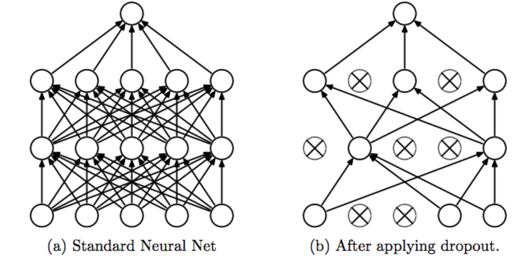
If we build a complicated neural network with lots of hidden layers and cells on a limited amount of training data, our model would probably memorize the data and does not generalize well. This phenomenon is called overfitting. Dropout is a regularizer to avoid overfitting by disabling some cells in hidden layers with some probability (Srivastava et. al. 2014). By doing this, dropout effectively samples from an exponential number of different networks in a tractable and feasible way. Dropout is computationally cheap and it can be applied in nearly any neural network architecture with ease. Wenn applying dropout, we basically do not change anything in our neural network in terms of optimization and model architecture. We only add a specific l2 weight regularisation term (which corresponds to choosing a prior) and dropout regularisation (which makes sampling from the posterior automatically) before each layer (input, hidden, output). Additionally, we need to apply dropout both in the training and test periods as opposed to its usual implementation. That’s all.
Yarin Gal tied up several derivations of stochastic variational inference to those of the stochastic regularization techniques, including dropout. Encouraged by this finding, he suggests to use dropout during test time in order to obtain approximate samples from the posterior function $p(\omega | x)$. When we apply dropout during test time, we obtain different results each time we run the model. They are approximate samples from the posterior predictive distribution. Gal calculates unbiased estimators for the mean and the variance of the posterior predictive distribution as the following:
Consider $y=f^{\hat{\omega}}(x)$ as the output of the Bayesian NN, and t= 1,.., T are samples from the posterior predictive distribution
\begin{equation} \mathop{\mathbb{\hat{E}}}(y)=\frac{1}{T}\sum_{t=1}^{T}f^{\hat{\omega_t}}(x) \end{equation}
\begin{equation} \mathop{\mathbb{\hat{E}}}(y^{T}y) = \tau^{-1}I + \frac{1}{T}\sum_{t=1}^{T}f^{\hat{\omega_t}}(x)^{T}f^{\hat{\omega_t}}(x) - \mathop{\mathbb{\hat{E}}}(y)^{T} \mathop{\mathbb{\hat{E}}}(y) \end{equation}
Note that $f^{\hat{\omega}}(x)$ is a row vector. The mean of our posterior predictive samples is an unbiased estimator of the mean of the approximate distribution $q(\omega)$. The sample variance plus a term $\tau^{-1}I$ is also an unbiased estimator of the variance of $q(\omega)$. That means, with only a small adjustment made to the sample variance, we get the Bayesian results very handy. The adjusting term $\tau$ equals to the following:
\begin{equation} \tau = \frac{(1-p)l^{2}}{2N\lambda} \end{equation}
N is the number of data points. $l$ is the prior lengthscale capturing our subjective belief over the prior’s frequency. A short length-scale $l$ corresponds to high frequency prior, and a long length-scale corresponds to low frequency prior. $\lambda$ corresponds to the weight decay regularization term which we additionally use to regularize weight optimization. As a trick during application we will play the equation above, and leave the $\lambda$ alone:
\begin{equation} \lambda = \frac{(1-p)l^{2}}{2N\tau} \end{equation}
The best $p$, $\tau$ and $\lambda$ can be found by cross-validation. They are the only paramteres to optimize when using the MC Dropout approach. It is a big relief considering the fact that sampling methods like MCMC and HMC usually require many parameters to optimize. After choosing $\lambda$, $p$ and $\tau$, all we need is to calculate the l2 weight-decay regularisation term $\lambda$ and apply this additional regularisation to our neural network model. Then we can calculate the statistical properties of our samples of posterior distribution in order to get new insights.
Data Exploration
For this tutorial, we aim to implement a Bayesian neural network using the MC Dropout technique to predict profit rates for the lending club loan data. Because a Bayesian neural network provides a distribution of probabilities, rather than a point estimate, we are able to use this distribution to then calculate measures including kurtosis, skewness, and variance. Later in this blog post, these measures will then be used to interpret the results.
Lending Club Loan Data
The lending club loan data set (accessible on kaggle.com: https://www.kaggle.com/wendykan/lending-club-loan-data) contains data for loans in the period of 2007 - 2015. It includes, among others, information about current payments, the loan status (current, late, fully paid etc.) and data about the borrower such as state, annual income and home ownership. The complete data set consists of approximately 890.000 rows and 74 columns.
Before we implement the Bayesian neural network, we will explore and clean the data. We are interested in past loans, therefore we have chosen only ‘Fully Paid’,‘Default’, or ‘Charged Off’ loans among all.
import pandas as pd
import seaborn as sns
import matplotlib.pyplot as plt
loan = pd.read_csv("data/loan.csv", low_memory=False)
loan = loan[loan.loan_status.isin(['Fully Paid','Default','Charged Off'])]
print(loan.shape)
loan.head()
(254190, 74)
| id | member_id | loan_amnt | funded_amnt | funded_amnt_inv | term | int_rate | installment | grade | sub_grade | ... | total_bal_il | il_util | open_rv_12m | open_rv_24m | max_bal_bc | all_util | total_rev_hi_lim | inq_fi | total_cu_tl | inq_last_12m | |
|---|---|---|---|---|---|---|---|---|---|---|---|---|---|---|---|---|---|---|---|---|---|
| 0 | 1077501 | 1296599 | 5000.0 | 5000.0 | 4975.0 | 36 months | 10.65 | 162.87 | B | B2 | ... | NaN | NaN | NaN | NaN | NaN | NaN | NaN | NaN | NaN | NaN |
| 1 | 1077430 | 1314167 | 2500.0 | 2500.0 | 2500.0 | 60 months | 15.27 | 59.83 | C | C4 | ... | NaN | NaN | NaN | NaN | NaN | NaN | NaN | NaN | NaN | NaN |
| 2 | 1077175 | 1313524 | 2400.0 | 2400.0 | 2400.0 | 36 months | 15.96 | 84.33 | C | C5 | ... | NaN | NaN | NaN | NaN | NaN | NaN | NaN | NaN | NaN | NaN |
| 3 | 1076863 | 1277178 | 10000.0 | 10000.0 | 10000.0 | 36 months | 13.49 | 339.31 | C | C1 | ... | NaN | NaN | NaN | NaN | NaN | NaN | NaN | NaN | NaN | NaN |
| 5 | 1075269 | 1311441 | 5000.0 | 5000.0 | 5000.0 | 36 months | 7.90 | 156.46 | A | A4 | ... | NaN | NaN | NaN | NaN | NaN | NaN | NaN | NaN | NaN | NaN |
5 rows × 74 columns
The first few rows of the data set show that some of the columns seem to have quite a lot of missing values. In order to obtain a better overview, we start by creating a data set loan_missing which contains boolean values for missing data. We then sum those missing values by column and calculate the percentage. Lastly, we order the dataframe by the percentage of missing values, with the highest percentage on top.
loan_missing = loan.isna()
loan_missing_count = loan_missing.sum()

loan_missing_percentage = (loan_missing_count / len(loan)).round(4) * 100
loan_missing_sorted = loan_missing_percentage.sort_values(ascending=False)
loan_missing_sorted.head(20)
annual_inc_joint               100.00
dti_joint                      100.00
verification_status_joint      100.00
il_util                         99.95
inq_last_12m                    99.94
mths_since_rcnt_il              99.94
open_acc_6m                     99.94
open_il_6m                      99.94
open_il_12m                     99.94
open_il_24m                     99.94
total_bal_il                    99.94
open_rv_12m                     99.94
open_rv_24m                     99.94
max_bal_bc                      99.94
all_util                        99.94
total_cu_tl                     99.94
inq_fi                          99.94
next_pymnt_d                    99.52
mths_since_last_record          87.48
mths_since_last_major_derog     81.17
dtype: float64
The resulting table proves that a lot of columns are almost completely empty. For further data exploration, we set a threshold of 50% and remove each column above this threshold. We now have 52 columns left.
temp = [i for i in loan.count()<len(loan)*0.50]
loan.drop(loan.columns[temp],axis=1,inplace=True)
loan.shape
(254190, 52)
Since there is no profit column existing in our data set yet, we define a target variable profit containing the profit rate of each loan. Then we have a look at the distribution of profits in order to find out if there are any imbalances in our target variable. We classify the target values as positive / negative profit and count the occurences in each class.
loan["profit_rate"] = loan.apply(lambda x: ((x['total_pymnt'] - x['loan_amnt'])/x['loan_amnt']), axis = 1)

target_class = pd.DataFrame(columns=["class"])
target_class["class"] = [1 if i > 0 else 0 for i in loan["profit_rate"]]
target_class["class"].value_counts()
1    207700
0     46490
Name: class, dtype: int64
The profit classes show that there are far more instances of positive profit than negative profit, meaning that our data set is imbalanced. But since we are going to apply a regression problem, this is less of an issue now. Now, we will have a look at what variables have the highest positive and negative correlation with our target variable.
loan.head()
corr = loan.corr()["profit_rate"].sort_values(ascending=False)
print('most positive correlations:\n', corr.head(10))

print('most negative correlations:\n', corr.tail(10))
most positive correlations:
 profit_rate         1.000000
total_rec_prncp     0.473400
total_pymnt         0.431424
total_pymnt_inv     0.428510
last_pymnt_amnt     0.290184
total_rec_int       0.196227
tot_cur_bal         0.052777
annual_inc          0.040834
total_rev_hi_lim    0.020487
revol_bal           0.004422
Name: profit_rate, dtype: float64
most negative correlations:
 total_rec_late_fee        -0.082807
dti                       -0.103913
int_rate                  -0.114446
out_prncp_inv             -0.131428
out_prncp                 -0.131428
id                        -0.164109
member_id                 -0.166208
collection_recovery_fee   -0.218884
recoveries                -0.351396
policy_code                     NaN
Name: profit_rate, dtype: float64
The columns total_rec_prncp (prinicpal received to date), total_pymnt (payments received to date for total amount funded) and total_pymnt_inv (payments received to date for portion of total amount funded by investors) have the highest positive correlation with our target column. The columnsout_prncp (remaining outstanding principal for total amount funded) and out_prncp_i (remaining outstanding principal for portion of total amount funded by investors) have the highest negative correlation with the target column. This certainly seems feasible for our past loans, but if we think about using the model for real world predictions, these variables may not be as significant.
loan["int_rate_dec"] = loan.apply(lambda x: (x["int_rate"]/100), axis = 1)
fig = plt.figure(figsize = (10,8))
ax1 = fig.add_subplot(221)
g = sns.distplot(loan["loan_amnt"], ax=ax1)
g.set_xlabel("Loan Amount", fontsize=12)
g.set_ylabel("Frequency", fontsize=12)
ax1.set_title("Loan Amount Distribution", fontsize=14)


ax2 = fig.add_subplot(222)
g1 = sns.distplot(loan['int_rate_dec'], ax=ax2)
g1.set_xlabel("Interest Rate", fontsize=12)
g1.set_ylabel("Frequency", fontsize=12)
ax2.set_title("Interest Rate Distribution", fontsize=14)


ax3 = fig.add_subplot(223)
g2 = sns.distplot(loan["profit_rate"])
g2.set_xlabel("Profit", fontsize=12)
g2.set_ylabel("Frequency", fontsize=12)
ax3.set_title("Profit Frequency Distribution", fontsize=14)

fig.tight_layout()
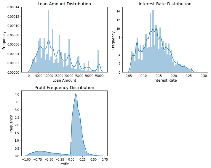
The above plots show the distributions of loan amount, interest rate and profit frequency. The majority of loans amount to 5.000 - 15.000$ each. Interest rates are mostly distributed between 0.10 - .20 %. The distribution of profit rates shows that there are only a few loans in the negative range. The profit distribution spikes between 0.00 - 0.25 %.
fig = plt.figure(figsize=(22,6))
sns.kdeplot(loan.loc[loan['profit_rate'] > 0, 'total_rec_prncp'], label = 'profit rate > 0')
sns.kdeplot(loan.loc[loan['profit_rate'] <= 0, 'total_rec_prncp'], label = 'profit rate <= 0');
plt.xlabel('Principal Received',fontsize=15)
plt.ylabel('Density',fontsize=15)
plt.title('Distribution of Principal Received to Date',fontsize=20);
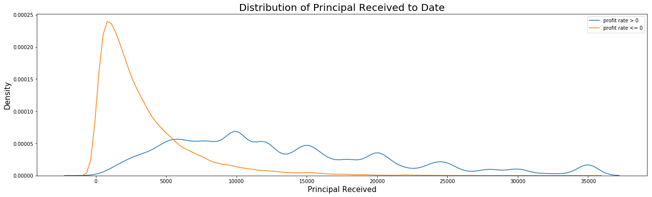
The distribution of principal received to date shows that most instances with negative profits appear in the range of 0 - 10,000$, whereas instances with positive profits are more widely distributed. Next, we will see if there are any borrowers who have taken more than one loan to see if their member ID could be an indicator of the profit rate.
loan['member_id'].value_counts().head()
5246974    1
1821228    1
1444503    1
922260     1
2417894    1
Name: member_id, dtype: int64
There are no members who have taken more than one loan. Consequently, the member id does not indicate whether the borrower is likely to pay back their loan. Hence, the column does not need to be considered for predictions.
profit_by_purpose = pd.DataFrame(loan[loan['profit_rate']>0].groupby('purpose')['profit_rate'].count().sort_values())
profit_by_purpose["profit_neg"] = pd.DataFrame(loan[loan['profit_rate']<=0].groupby('purpose')['profit_rate'].count().sort_values())["profit_rate"]

fig, ax = plt.subplots(figsize=(14, 10))
profit_by_purpose.plot(kind="bar", ax=ax)
plt.ylabel('Number of loans',fontsize=15)
plt.xlabel('Purpose',fontsize=15)
plt.title('Number of loans by purpose', fontsize=20);
L=plt.legend()
L.get_texts()[0].set_text('positive profit')
L.get_texts()[1].set_text('negative profit')
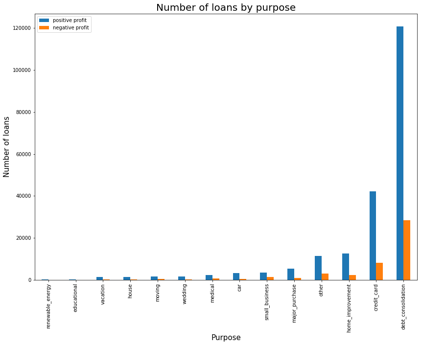
The barplot shows the number of loans issued per purpose category. Most loans are issued for debt consolidation and credit cards - these are also the categories with the highest amount of loans with negative profit. There is no category where the amount of loans with negative profits exceeds loans with positive profits. However, there certainly are categories where the share of negative profits is very small, such as house, car or wedding.
Returning back to data preprocessing, we applied a feature selection by temporarily recasting the regression problem as a binary decision problem between positive and negative profit rates. Then we calculated Information Value for all columns. Nevertheless, there were many columns in our dataset that can be influenced by the target variable. Therefore, we selected only the useful, but not too predictive variables.
features = loan[['annual_inc','int_rate','purpose','dti','term','grade']]
features = pd.get_dummies(features)
target = loan[['profit_rate']]
In order to obtain comparable and reliable results, we have sampled 100k rows from the remaining dataset and split it into a test set with 33k rows, and a training set with 67k rows. To do this, we use the train_test_split() function by sklearn. Furthermore, we used the profit rate we have calculated before as our target variable.
import random
random.seed(100)
idx = random.sample(range(features.shape[0]), 100000)
f_sampled = features.iloc[idx,:]
t_sampled = target.iloc[idx]
import warnings
warnings.filterwarnings('ignore')
from sklearn.model_selection import train_test_split
from sklearn import preprocessing
import numpy as np

X_train, X_test, y_train, y_test = train_test_split(f_sampled, t_sampled, test_size=0.33, random_state=42)

scaler_trx = preprocessing.StandardScaler().fit(X_train)
X_train = scaler_trx.transform(X_train)

scaler_try = preprocessing.StandardScaler().fit(y_train)
y_train = scaler_try.transform(y_train)

scaler_testx = preprocessing.StandardScaler().fit(X_test)
X_test = scaler_testx.transform(X_test)

scaler_testy = preprocessing.StandardScaler().fit(y_test)
y_test = scaler_testy.transform(y_test)
Model
import pandas as pd
from keras import Model as Model
from keras import Input as Input
from keras.layers import Dropout
from keras.layers import Dense
from keras.regularizers import l2
from sklearn.metrics import mean_squared_error
import numpy as np
Using TensorFlow backend.
The following function defines the architecture of our model. It passes the following four parameters:
- n_hidden: a vector containing the number of neurons for each hidden layer
- input_dim: the number of input dimensions, which is equal to the number of columns in our training set
- dropout_prob: the dropout probability for the dropout layers in the neural network. The value should usually be between 0.05 - 0.5
- reg: used for regularization during MC Dropout
Next, we instantiate our model. The dropout technique is usually done only during training, but not during test time. Therefore, the usual Keras Sequential() model automatically switches off the dropout during test time. In order to get around this issue, we build a functional model in Keras. We start with the input layer using the Keras Input() function and pass the input dimensions. Using Dropout(), we apply the dropout technique to our inputs. Lastly, we instatiate a regular densely-connected layer using the Dense() function. Here we pass the dimensionality as an argument using the first value of the n_hidden vector. We use the tanh activation function and pass the regularization function, which will be explained in more detail below. We use a weight regularizer (called W_regularizer), with the l2 weight regularization penalty - this corresponds to the weight decay.
Now, for each hidden layer (using the length of the n_hidden vector), we instantiate the dropout function and a dense layer, as described above. Lastly, we create the output layer in the same way. The dimensionality of our output layer is one, since we only predict one target variable - the profit rate.
def architecture(model_type, n_hidden, input_dim, dropout_prob, reg):

    inputs = Input(shape=(input_dim,))
    inter = Dropout(dropout_prob)(inputs, training=True)
    inter = Dense(n_hidden[0], activation='tanh',
                  W_regularizer=l2(reg))(inter)
    for i in range(len(n_hidden) - 1):
        inter = Dropout(dropout_prob)(inter, training=True)
        inter = Dense(n_hidden[i+1], activation='tanh',
                      W_regularizer=l2(reg))(inter)
        inter = Dropout(dropout_prob)(inter, training=True)
        outputs = Dense(1, W_regularizer=l2(reg))(inter)
        model = Model(inputs, outputs)
    return model
In the following step, we define a function that runs our model. Before we do so, we pre-process our test data so we can use it as a default argument for our predictions.
The function model_runner() takes the following arguments:
- X_train/y_train: the training data
- X_test/y_test: the test data, using the 40k test set as a default
- dropout_prob: the dropout probability, which is then passed on to the model
- n_epochs: the number of epochs
- tau: tau value used for regularization
- batch_size: the size of the batches used for fitting the model
- lengthscale: the prior length scale
- n_hidden: a vector containing the number of neurons per layer, which is passed on to the model as well
We now define the input dimension to equal the number of columns in the training set. We also define a value N, which corresponds to the number of rows in the training set and is used for the regularization function. The regularization is carried out in a variable reg. The regularization function used here is the same function we introduced in the theory part, section Monte Carlo Dropout. Now we simply build the model using the architecture() function implemented above. Compile() configures the model for training. We then train our model using the function fit(), where we pass our training data, as well as the batch size and the number of epochs. The argument verbose = 1 results in a progress bar being shown during training. We keep it 0 for now to save spacing.
def model_runner(X_train, y_train,
                dropout_prob=0.20, n_epochs=100, tau=1.0, batch_size=500,
                lengthscale=1e-2, n_hidden=[100,100]):

    input_dim = X_train.shape[1]
    N = X_train.shape[0]
    reg = lengthscale**2 * (1 - dropout_prob) / (2. * N * tau)


    print('McDropout NN fit')

    model_mc_dropout = architecture(model_type = 'mcDropout',
                                    n_hidden=n_hidden, input_dim=input_dim,
                                    dropout_prob=dropout_prob, reg=reg)
    model_mc_dropout.compile(optimizer='sgd', loss='mse', metrics=['mae'])
    model_mc_dropout.fit(X_train, y_train, batch_size=batch_size, nb_epoch=n_epochs, verbose=0)


    return model_mc_dropout
Prediction
It is now time to use the model to make predictions. We implement another function called predictor(), which takes the following arguments:
- model_mc_dropout: the dropout model
- X_test/y_test: the test data
- T: the number of predictions made for each observation
We now use T in a for loop to run the predictions as many times as we specified. The results are added to a list called probs_mc_dropout. This results in a two-dimensional list with T items in each list. In other words, for each row in the test set, we now have a set of T predictions, enabling us to calculate uncertainty, and other measures such as variance, mean or skewness.
def predictor(model_mc_dropout,
              X_test = X_test, y_test = y_test, T = 100):
    probs_mc_dropout = []
    for _ in range(T):
        probs_mc_dropout += [model_mc_dropout.predict(X_test,verbose=0)]
    predictive_mean = np.mean(probs_mc_dropout, axis=0)
    predictive_variance = np.var(probs_mc_dropout, axis=0)
    mse_mc_dropout = mean_squared_error(predictive_mean, y_test)
    print(mse_mc_dropout)

    return probs_mc_dropout
Results and Evaluation
In the introduction it was mentioned that we are going to use Sharpe Ratio adjusted for skewness and kurtosis as a measure of loan application “goodness”.
The Sharpe Ratio (Sharpe (1966)) is defined as:
$SR = \frac{r - i}{SD}$
where r stands for expected return (in our case mean of the distribution), i for risk free interest rate (we assumed it is 0), and SD for standard devition, as a measure of a risk.
However, as it was explained in the introduton, normal distribution of profit rates seems as unnecessary strong assumption. Hence, Sharpe Ratio, accounting just for mean and variance, is unsuitable.
In order to solve this we employ adjustment introduced by Pezier and White (2006), where in addition to mean and standard deviation, we take into account skewness and kurtosis of distribution. Additionally, it should be mentioned that the following formula assumes exponential utility function and further risk-seeking behaviour of economic agents. This assumption seem quite reasonable in our case. The Adjusted for Skewness and Kurtosis Sharpe Ratio (ASKSR):
$ASKSR = SR[1 + \frac{S}{6}SR - \frac{K - 3}{24} SR^{2}]$
Where K stands for kurtosis and S for skewness.
Now let’s see how our models perform. We calculated ASKSR for each applicant in our test dataset of 33k observations. Then, on the first half of the test dataset, we found an optimal cutoff point for ASKSR. We did it by summing the profit that is above some assumed ASKSR level. Then, we evaluate the optimal cutoff on the second part of the test sample. We are expressing the result as a percantage of the maximum possible profit (i.e. sum of possitive profits). The ASKSR is evaluated for MC Dropout and Variational Inference. As a benchmark three measures are used: maximal profit (in case of a perfect prediction so that all profits are positive)m naive profit (the actual profit from the dataset), and the profit from deterministic feed-forward neural network. In the case of the last one we look for the profit-maximizing cut-off as well.
import pickle
import numpy  as np
from scipy.stats import kurtosis, skew, mode
import pandas as pd
from sklearn.model_selection import train_test_split
import glob
The following function helps us find the profit-maximizing cut-off. The arguments are x and y, for the cutoff array and profit arrey, respectively.
def optimalCut (x,y):
        max_y = max(y)
        max_x = x[y.index(max_y)]
        return (max_x)
Now, we load the absolute profit (real values) defined as the difference between total payment and the loan amount:
profit = np.array(pickle.load(open( "data/y_test_abs.pickle", "rb" )))
Next, we are using those 100 predictions per application to find the shape measures of distribution- mean, variance, skewness, and kurtosis. ASKSR is calculated and optimal cut-off point is found. We decide to accept all the loans above this level of ASKSR. First we calculate the results of MC Dropout, than Variational Inference, and, finally, the results from deterministicly weighted Neural Network.
method = []
stacked_res = []

results = np.array(pickle.load(open( "results/bayesian/mc_dropout.pickle", "rb" )))

df = pd.DataFrame(
     {'mean': np.mean(results, axis=0)[:,0],
      'variance': np.var(results, axis=0)[:,0],
      'skewness': skew(results, axis = 0)[:,0],
      'kurtosis': kurtosis(results, axis = 0)[:,0],
      'Returns': profit
     })

df['standardDeviation'] = np.sqrt(df['variance'])
df['SR_mean'] = df['mean']/df['standardDeviation']
df['ASKSR_mean'] = df['SR_mean'] * (1 + df['skewness'] * df['SR_mean']/6 - (df['kurtosis'] - 3)/24 * (df['SR_mean'] ** 2))


df, df_test = train_test_split(df, test_size=0.5, random_state=42)

ASKSR_cutoff_mean = np.linspace(min(df['ASKSR_mean']), max(df['ASKSR_mean']), 10000)

ASKSR_profit_mean = []

for i in range(0, len(ASKSR_cutoff_mean) - 1, 1):
    ASKSR_profit_mean.append(df.loc[df['ASKSR_mean'] > ASKSR_cutoff_mean[i], 'Returns'].sum())


ASKSR_mean_Optimal = optimalCut(x = ASKSR_cutoff_mean, y = ASKSR_profit_mean)

ASKSR_profit_optimal_mean = []
ASKSR_profit_optimal_mean.append(df_test.loc[df_test['ASKSR_mean'] > ASKSR_mean_Optimal, 'Returns'].sum())

method.append("MC Droput")
stacked_res.append(ASKSR_profit_optimal_mean)
results = np.array(pickle.load(open( "results/bayesian/VariationalInference.pickle", "rb" )))

df = pd.DataFrame(
    {'mean': np.mean(results, axis=0),
    'variance': np.var(results, axis=0),
    'skewness': skew(results, axis = 0),
    'kurtosis': kurtosis(results, axis = 0),
    'Returns': profit
    })

df['standardDeviation'] = np.sqrt(df['variance'])
df['SR_mean'] = df['mean']/df['standardDeviation']
df['ASKSR_mean'] = df['SR_mean'] * (1 + df['skewness'] * df['SR_mean']/6 - (df['kurtosis'] - 3)/24 * (df['SR_mean'] ** 2))


df, df_test = train_test_split(df, test_size=0.5, random_state=42)

ASKSR_cutoff_mean = np.linspace(min(df['ASKSR_mean']), max(df['ASKSR_mean']), 10000)

ASKSR_profit_mean = []

for i in range(0, len(ASKSR_cutoff_mean) - 1, 1):
    ASKSR_profit_mean.append(df.loc[df['ASKSR_mean'] > ASKSR_cutoff_mean[i], 'Returns'].sum())


ASKSR_mean_Optimal = optimalCut(x = ASKSR_cutoff_mean, y = ASKSR_profit_mean)

ASKSR_profit_optimal_mean = []
ASKSR_profit_optimal_mean.append(df_test.loc[df_test['ASKSR_mean'] > ASKSR_mean_Optimal, 'Returns'].sum())

method.append("Variational Inference")
stacked_res.append(ASKSR_profit_optimal_mean)
results = np.array(pickle.load(open( "results/deterministic/Regularized.pickle", "rb" )))

df = pd.DataFrame(
        {'mean': results[:,0],
         'Returns': profit
        })

df, df_test = train_test_split(df, test_size=0.5, random_state=42)

deterministic_cutoff_mean = np.linspace(min(df['mean']), max(df['mean']), 10000)

deterministic_profit_mean = []

for i in range(0, len(deterministic_cutoff_mean) - 1, 1):
    deterministic_profit_mean.append(df.loc[df['mean'] > deterministic_cutoff_mean[i], 'Returns'].sum())

deterministic_mean_Optimal = optimalCut(x = deterministic_cutoff_mean, y = deterministic_profit_mean)

deterministic_profit_optimal_mean = []
deterministic_profit_optimal_mean.append(df_test.loc[df_test['mean'] > deterministic_mean_Optimal, 'Returns'].sum())

method.append("Deterministic")
stacked_res.append(deterministic_profit_optimal_mean)
Including naive and maximum profit as benchmarks:
method.append("Naive")
stacked_res.append(sum(df_test['Returns']))

method.append("Max")
stacked_res.append(df_test.loc[df_test['Returns'] > 0, 'Returns'].sum())
results_Compare = pd.DataFrame(
        {'method': method,
         'result': stacked_res
        })
results_Compare
| method | result | |
|---|---|---|
| 0 | MC Droput | [6003450.44596908] |
| 1 | Variational Inference | [5744692.21274037] |
| 2 | Deterministic | [5907009.12064385] |
| 3 | Naive | 949249 |
| 4 | Max | 2.55511e+07 |
for j in range (0,3):
    results_Compare['result'][j] = results_Compare['result'][j][0]
for m in range (0,4):
    results_Compare['result'][m] = results_Compare['result'][m]/results_Compare['result'][4]
Finally, results. They are expressed as a share of the maximal profit.
results_Compare
| method | result | |
|---|---|---|
| 0 | MC Droput | 0.234959 |
| 1 | Variational Inference | 0.224832 |
| 2 | Deterministic | 0.231184 |
| 3 | Naive | 0.037151 |
| 4 | Max | 2.55511e+07 |
We can see that compared to the naive approach, all three Neural Network based approaches provide a significant increase in profit- by almost 20%. MC Dropout beats both deterministic approach and VI by a margin, while all three are way better than naive approach. All results are obtained from neural networks of the same architecture, 2 hidden layers each with 100 cells.
It should be noted, however, that the measures derived from Bayesian approaches (ASKSR) and the deterministic one (predicted profit rate) are not fully comparable. Hence, this result should be take with a grain of salt. For better and more definite results we propose using bigger training datasets as well as including more traditional methods, with a more solid theoretical support, for Bayesian approximation, such as Hamiltonian Monte Carlo or Markov Chain Monte Carlo (MCMC).
Conclusion
In this study, we attempted to show that uncertainty is not only something that places obstacle in front of good predictions. We can indeed benefit from it, if we are able to estimate it. It is a difficult task though. Approximate Bayesian variational inference techniques provide us with scalable estimations. Among them, MC dropout yields results those are very close to usual neural network models in performance. MC dropout is easier to use, faster and more scalable. We apply dropout very intuitively on both training and test times and automatically obtain an approximate probabilistic model. But it is just one way of approximating the posterior. Applications of Bayesian inference in deep learning is a reviving field, and now in development. In near future, we are likely to witness better theoretical explorations and algorithmic developments. Not to say further successful applications in finance and many other fields.
Bibliography
- Knight, F. (1921). From Risk, Uncertainty, and Profit. The Economic Nature of the Firm.
- Gal., Y. (2015, July 3). What My Deep Model Doesn’t Know [Web log post]. Retrieved February 8, 2017, from http://mlg.eng.cam.ac.uk/yarin/blog_3d801aa532c1ce.html
- Bernardo, J. M., & Smith, A. F. (1994). Bayesian Theory. Wiley Series in Probability and Statistics.
- Neal, R. M. (1996). Bayesian Learning for Neural Networks. Lecture Notes in Statistics.
- Betancourt, M., & Girolami, M. (2015). Hamiltonian Monte Carlo for Hierarchical Models. Current Trends in Bayesian Methodology with Applications. doi:10.1201/b18502-5
- Robert, C. P., & Casella, G. (2004). Monte Carlo Optimization. Springer Texts in Statistics Monte Carlo Statistical Methods.
- Murphy, K. P. (2012). Machine learning: A probabilistic perspective. Cambridge, England: The MIT Press.
- Graves, A. (2011). Practical variational inference for neural networks. Advances in Neural Information Processing Systems.
- Ranganath, R., Gerrish, S., & Blei, D. M. (2014). Black Box Variational Inference. Proceedings of the 17th International Conference on Artificial Intelligence and Statistics (AISTATS), 33.
- Blei, D. M., Kucukelbir, A., & Mcauliffe, J. D. (2017). Variational Inference: A Review for Statisticians. Journal of the American Statistical Association, 112(518), 859-877.
- Gal, Y., & Ghahramani, Z. (2016). Dropout as a Bayesian Approximation: Representing Model Uncertainty in Deep Learning. Proceedings of the 33 Rd International Conference on Machine Learning, 43.
- Srivastava, N., Hinton, G., Krizhevsky, A., Sutskever, I., & Salakhutdinov, R. (2014). Dropout: a simple way to prevent neural networks from overfitting. Journal of Machine Learning Research, 15 (1).
- MacKay, D. J. (2004). Information theory, inference, and learning algorithms. Cambridge, U.K.: Cambridge University Press.
- Osband, I. (2016). Risk versus Uncertainty in Deep Learning : Bayes , Bootstrap and the Dangers of Dropout.
- Sharpe, W. F. (1966). “Mutual Fund Performance”. Journal of Business. 39 (S1): 119–138.
- Pezier J, & White A, (2006) “The relative Merits of Investable Hedge Fund indices and of Funds of Hedge Funds in Optimal Passive Portfolios”
- Andreeva, G., Ansell, J., & Crook, J. (2007). Modelling profitability using survival combination scores. European Journal of Operational Research, 183, 1537-1549.
- R T Stewart (2011) A profit-based scoring system in consumer credit: making acquisition decisions for credit cards, Journal of the Operational Research Society, 62:9, 1719-1725, DOI: 10.1057/jors.2010.135
- S M Finlay (2008) Towards profitability: a utility approach to the credit scoring problem, Journal of the Operational Research Society, 59:7, 921-931, DOI: 10.1057/ palgrave.jors.2602394
- Luis Javier Sánchez Barrios, Galina Andreeva & Jake Ansell (2014) Monetary and relative scorecards to assess profits in consumer revolving credit, Journal of the Operational Research Society, 65:3, 443-453, DOI: 10.1057/jors.2013.66
- Carlos Serrano-Cinca-Begoña Gutiérrez-Nieto (2016), The use of profit scoring as an alternative to credit scoring systems in peer-to-peer (P2P) lending, Decision Support Systems, https://doi.org/10.1016/j.dss.2016.06.014
- Thomas Verbraken, Cristian Bravo, Richard Weber, Bart Baesens (2014), Development and application of consumer credit scoring models using profit-based classification measures, European Journal of Operational Research
- Stefan Lessmann, Bart Baesens, Hsin-Vonn Seow, Lyn C. Thomas (2015), Benchmarking state-of-the-art classification algorithms for credit scoring: An update of research, European Journal of Operational Research
- Mee Chi So, Lyn C. Thomas, Hsin-Vonn Seow, Christophe Mues (2014), Using a transactor/revolver scorecard to make credit and pricing decisions, Decision Support Systems
- Kaveh Bastani, Elham Asgari, Hamed Namavari (2018), Wide and Deep Learning for Peer-to-Peer Lending, arXiv
- Selçuk Bayracı (2017), Application of profit-based credit scoring models using R, Romanian Statistical Review 4/2017
- Devavrat Shah and Kang Zhang (2014), Bayesian regression and Bitcoin, 52nd Annual Allerton Conference on Communication, Control, and Computing (Allerton)
- Catarina Moreira and Emmanuel Haven and Sandro Sozzo and Andreas Wichert (2017), The Dutch’s Real World Financial Institute: Introducing Quantum-Like Bayesian Networks as an Alternative Model to deal with Uncertainty, arXiv
- Michael Maio Pires and Tshilidzi Marwala (2007), Option Pricing Using Bayesian Neural Networks, arXiv