Authors: Christopher Ketzler, Stefan Grosse, Raiber Alkurdi

Motivation

The development of machine learning or deep learning (ML/DL) models which provides the user to have a decision to a specific problem has progressed enormously in the last years. The emergence of better computer hardware and therefore software, and the collecting of big data leads to more and more complicated algorithms. If these algorithms are no more understandable by average humans in terms of what are they doing or why they give a certain decision, we call them black-boxes.

In this blog we want to focus on why it is so important to understand these seemingly accurate decision systems instead of only accept the good performance and blindly use them. We provide the reader with theoretical approaches to examine this problem and deliver some practical connections to it with a selected dataset and present some models to explain the black-boxes by using python programming language.

1. Introduction

Black-boxes seem to influence our life more and more. Nowadays machine learning algorithms are used in many parts of the economy, society and even in politics. But what is the problem? The data from which the learning algorithms get the information, can consists of natural prejudices and biases or is intentionally manipulated, what can lead to wrong decisions with large effects. This problem is a problem of white box systems as well but, we are able to protect and react against it because we understand them. When a system, which we cannot explain in functionality and the reasons for having a certain result, is used in the open environment, then it is getting very complicated in terms of business decisions, documentary report of a model, law interpretation and the general trust and acceptance. So, we are faced with the problem that such practices and prejudices are unconsciously considered as general rules and we have a tradeoff between interpretability and accuracy.

Increasingly more countries starting to implement laws, regulating the use and liability issues of black-box system because they are respected as mighty methods, e. g. the European Union, who introduce the right to explanation, which gives a user the possibility of an explanation from an automated decision system [1,2]. Also, the investments for development and application in this field rise, e.g. the German government has recently decided to put three billion euros into artificial intelligence and emphasized that this is a task for the whole society and that the technologies need to be understood [3]. There are a lot of interesting examples which shows how the systems can be fooled, humans misinterpret results or the danger that can occur [4,5]. But one should not forget the great possibility to gain new knowledge in terms of e.g. unknown coherence in data due to the explanation of black-boxes. In many parts of our life, these automated decision systems already helping us doing a lot of work and there is a trend towards more automation. With the rise of artificial intelligence, which of cause is based on such algorithms, this issue will be the key discussion for the future.

2. Theoretical and technical foundations

The target for this part of the blog is to give the reader an overview of the most importance approaches to explaining black-box systems, we want to mention the major properties for this field of research and at the end, offer an answer to the state-of-the-art question.

Like the development of black-box models is a recent issue, the explanation of them is even newer. For this reason, the relevant literature is continuous developing and is not established like we know it from other fields in research. Therefore, in this part of the blog we based our explanations and simultaneously we want to recommend to the paper of Guidotti, R. et al. [4], which gives the reader a deep insight into the topic and supports with a structured categorization what it makes much easier to understand the problems we are faced with by working in this area.

2.1. Basics - General assumptions

Black-box systems can be very different in their inner complexity, what means e.g. that the response functions can be non-linear and non-monotonic and so on. Because we cannot look into the black-box, we need to assume the highest complexity, and the more complex a black-box is, the harder a satisfying explanation should be. In our fast-moving world we are often faced with situations where a rapid solution or overview is needed. Therefore, it can be advantageous to have a less detailed explanation without putting too much effort into it. Otherwise, in very sensitive cases a much more detailed explanation is needed and in general these explanations require a higher foreknowledge of the user. The authors named the problem of time as Time Limitation and the knowledge of the users as Nature of User Expertise [4]. With respect to these properties and to our actual task to open a black-box, we assume that the analysis of the data itself or the preprocessing step, where some problems can be solved beforehand, will not be considered here.

2.2 Interpretability - Global / Local

The human eyes and mind are some very powerful instruments to interpret images (IMG) or texts (TXT) even better as a machine, at least until now. Nevertheless, it is absolutely useful to have systems, which are much faster, to get the job done and it is established practice to use them. We are still able to have a look on a result and correct a system when sensitive decisions have to be done. But when it comes to complex tabular dataset (TAB), we are no more able to handle it. Due to that properties, it makes sense that many explanation systems offer a visual or textual representation of an explanation. Therefore, we will be continuing not to leave out the consideration of text and image data but when it comes to our examples later on, our focus is set on tabular data.

It is important to clarify what is meant by explaining a black-box or the actual definition of the word interpretability. As we learned from [4], in the literature the term interpretability is widely discussed and is split up in many dimensions and unfortunately it is not possible to measure it. It is important to see, that interpretability should be connected with causality, trust or fidelity and not only understanding [6,7], and with the respect of the user expertise, interpretability can be a very subjective term. What exactly should be explained, the reasons for a specific outcome, internal workings or a general behavior? Ideally, we want answers to all these questions and a transparency, like we know it from e.g. a simple linear, monotonic relationship between dependent and independent variables, is hard to realize. To remember the definition of a black-box can help to see that is a very difficult task. Some important aspects to increase trust in black-box is e.g. transferability, the ability to transfer findings to a common model, otherwise we can be affected by a change over time of the relationship between input and output variables [8]. Robustness, how is the black-box able to handle perturbations in the data, and especially for black-boxes, how the model behaves by changing the input data [8]. A black-box can have so many artefacts or e.g. can be connected with external sources, that it would need infinity test sets to check on them. The key take-away here is that a black-box system should be interpretable what leads to comprehensibility and trust in it, and that this is the focus of ongoing research.

Now we come to the first categorization which brings an order into the already existing methods to explain black-boxes. We can explain a black-box as a whole or just interpret specific parts of it. The first describes the global interpretability, which gives an explanation of the entire model and the logic of its behavior, e.g. what influences the returning of an item in an online store. Whereas local interpretability provides us with explanation for only one specific case of decision outcome, e.g. what influences the returning of an item of Person X, which of cause can be different from the global reasons. In general, you can say that a local explanation is more precise than a global one because, you can expect the behavior to be more linear and monotonic when looking at a smaller part of the model as if you want to approximate the entire model.

2.3 Reverse engineering

A general difficulty is, that the training dataset from which a black-box learned, can be not available. We can see this situation as a worst case but a real-world scenario. Of cause, it is possible to examine a blank black-box which is trained for the first time by our training dataset, the explanation approach stays the same. Post-hoc interpretability or reverse engineering is widely used in the literature and is the main approach to explain a black-box [4,8]. This means, we are provided with the black-box predictor which learned from a dataset and we only can observe the predictions for an input dataset, so we only can explain the black-box after giving a decision. The task of the explanator method is to mimic the behavior of the black-box with a so-called oracle dataset. This oracle dataset is the combination of the input dataset and their prediction. To clarify this procedure, see Figure 1.

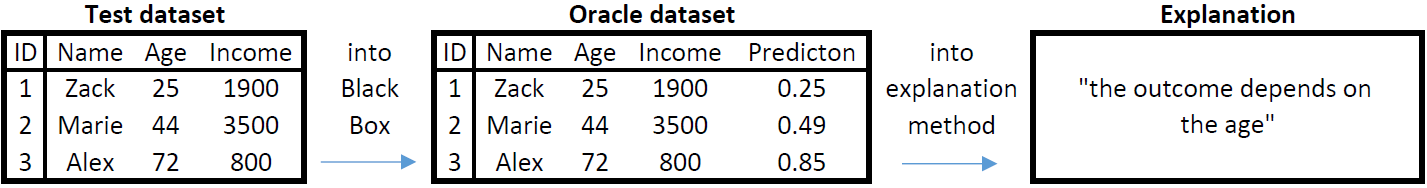
Figure 1 - Reverse engineering - creating an Oracle dataset for an explanation

A property for some explanator methods is, that they can used for every kind of black-box system e.g. Neural Network (NN), Tree Ensemble (TE), Support Vector Machines (SVM), Deep Neural Network (DNN). This feature is named agnostic (AGN) and has some advantages and disadvantages e.g. with respect for the matters of time limitation and the expertise problem. The agnostic approach, also called generalizable, is only observing the changes in the oracle dataset without looking on special or internal properties of the black-box e.g. a distance measures between trees in a random forest [4]. In general, to extract internals of a black-box, especially for sensitive applications, are necessary to get a deep understanding and an explanation method who concentrates on a specific black-box can be more useful. On the other side, an agnostic approach can save a lot of time and brings faster results which are maybe easier to understand.

2.4 Design of explanation – Problem identification

Due to fact that meanwhile a lot of state-of-the-art methods exist which addressing different sets of problems, Guidotti, R. et al. [4] try to bring an order into it. The Authors dividing all methods into three parts concerning the how in general they work or what problem they will solve. In the following we explaining these three parts.

The model explanation problem describes methods which are able to give a global interpretation of a black-box system. Figure 2 describes this mechanism. At first the user needs a test dataset, here called test instances, to feed the already trained black-box and produce their predictions. After that we are able to mimic the behavior of the black-box with the actual predictor or explanation model, here interpretable global predictor, and receive an understandable result of the whole logic of the black-box. So, it explains how the overall logic behind the black-box works.

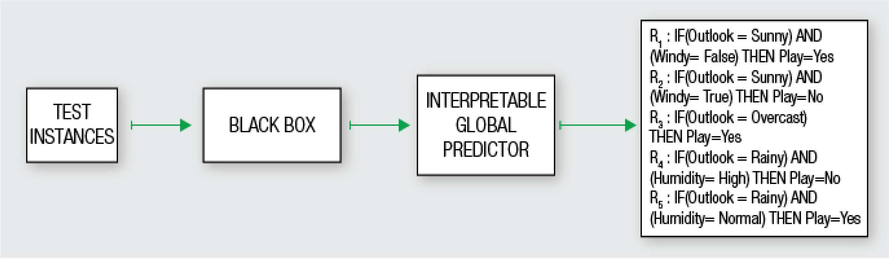Figure 2 - Model explanation problem - Source: Guidotti, R. et al. [4]

The outcome explanation problem describes methods which are able to give a local interpretation of a black-box system. Figure 3 describes this mechanism. It is the same procedure like above but we receive an understandable prediction-result of a specific instance of the test dataset.

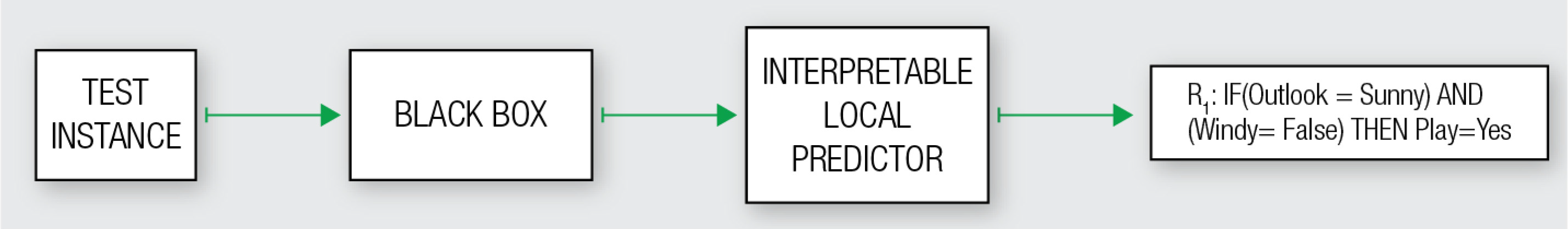
Figure 3 - Outcome explanation problem - Source: Guidotti, R. et al. [4]

The model inspection problem describes methods concentrates on the analysis of specific properties of the black-box. These methods providing a textual or visual explanation of for example identifying specific neurons or looking on the impact of changes in a variable. So, they show how the black-box work internally. Figure 4 describes this mechanism. Again, it is the same procedure, but now we are provided with a e.g. visual representation of how the black-box work internally.

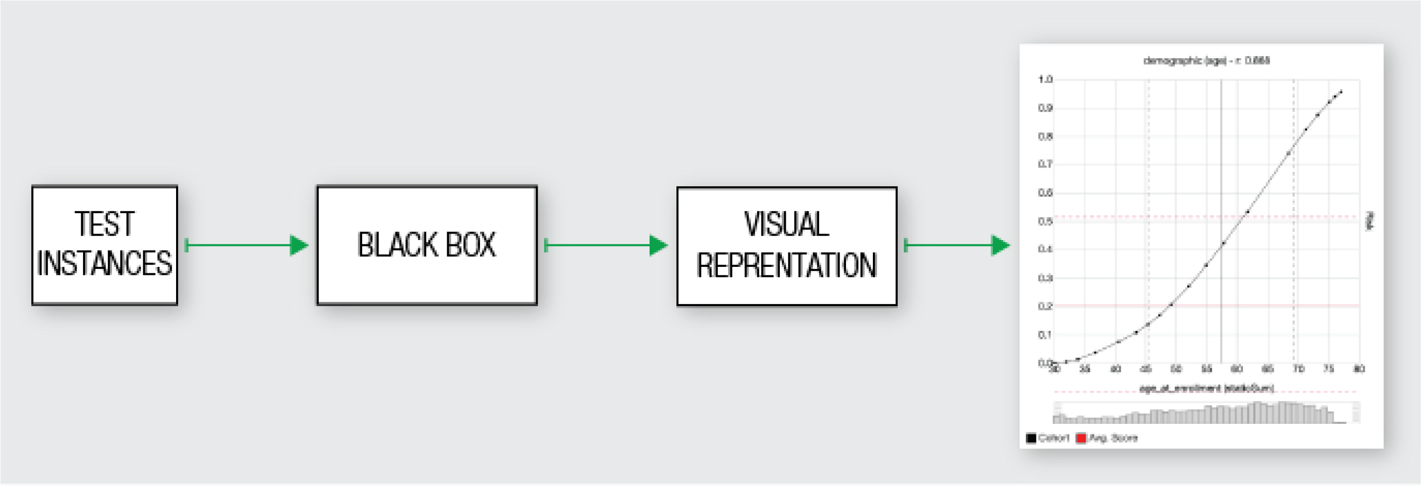
Figure 4 - Model inspection problem - Source: Guidotti, R. et al. [4]

2.5 The explanators

Here we support the reader with a listing of the explanators used in explanation systems and some descriptions. These explanators in general are interpretable or offering a textual or visual description of a black-box. The main idea is to find an explanation model, which is an interpretable approximation of the original complex black-box or to reveal some inner workings. If this interpretable model gives a valuation or shows behaviors which one expected to be comprehensible compared to the black-box, it might be increasing trust. In general, the explanators has many different variations in functionality and/or for different uses. Therefore, we again want to refer to [4] because a short description of all methods is given.

Features Importance (FI) - for detailed explanation see Example 1

Partial Dependence Plot (PDP) - for detailed explanation see Example 2

Decision Tree (DT) and Decision Rules (DR) are known in general as interpretable representations and the main problem solver for the model explanation problem for tabular data and any kind of black-box. They are able to give an approximation of the behavior on a global scope. But when it comes to very complex black-box system, the danger is that the explanations from these explanators indeed mimic the black-box very good, but the results are so complex that they are no more interpretable, e.g. an output of many sites full of decision rules or a too deep tree [4]. Some of these methods offer an evaluation of the interpretable predictor, which compares the accuracy of the original black-box with the accuracy of the understandable method. For a detailed description how to interpret black-box models with single tree approximation we refer to [9].

Sensitivity Analysis (SA) a state-of-art-tool for the model inspection problem and advisable to use when a better understanding of a black-box is required. It produces a visual representation to robustness of a model, by looking how the output changes for changing the inputs with sensitivity samples. For a more detailed explanation we refer to [10] and for a self-use with programming code we recommend the Sensitivity Analysis Library for Python SALib [11].

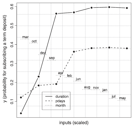
Figure 5 - Sensitivity Analysis - shows the effect on the probability to subscribe to a term deposit by changing the input vaues of the three variables with the most influence - Source: Cortez, P. et al. [10]

Saliency Mask (SM) is a common tool for the outcome explanation problem and model inspection problem, mainly for image data used in a DNN. Therefore, some approaches take special properties of the black-box into account. It is a visual representation of a certain outcome and highlighting the cause of and e.g. a probability measure of it. For detailed explanations we refer to [12].

Figure 6 - Saliency Mask - Shows the area of attention - Source: Fong, R. C. et al. [12]

Activation Maximization (AM) a solver for the model inspection problem for (deep) neuronal networks for images to reveal inner workings of them. The aim is to find the neurons which are responsible for a decision. Activation maximization also can be used to see the reasons of a result like Saliency Mask.

2.6 Explaining models - Classification

From the aforementioned basics, it is now possible to display an overview of important explanation models, sorted by the three different problems mentioned above. This overview shows the main references. In Guidotti, R. et al. [4] you can see a more detailed overview and further overviews with extensions of the main references.

Name	Authors	Problem	Explanator	Black-Box	Data Type
Trepan	Craven et al.	Model Expl.	DT	NN	TAB
-	Krishnan et al.	Model Expl.	DT	NN	TAB
DecText	Boz	Model Expl.	DT	NN	TAB
GPDT	Johansson et al.	Model Expl.	DT	NN	TAB
Tree Metrics	Chipman et al.	Model Expl.	DT	TE	TAB
CCM	Domingos et al.	Model Expl.	DT	TE	TAB
-	Gibbons et al.	Model Expl.	DT	TE	TAB
TA	Zhou et al.	Model Expl.	DT	TE	TAB
CDT	Schetinin et al.	Model Expl.	DT	TE	TAB
-	Hara et al.	Model Expl.	DT	TE	TAB
TSP	Tan et al.	Model Expl.	DT	TE	TAB
Conj Rules	Craven et al.	Model Expl.	DR	NN	TAB
G-REX	Johansson et al.	Model Expl.	DR	NN	TAB
REFNE	Zhou et al.	Model Expl.	DR	NN	TAB
RxREN	Augasta et al.	Model Expl.	DR	NN	TAB
SVM+P	Nunez et al.	Model Expl.	DR	SVM	TAB
-	Fung et al.	Model Expl.	DR	SVM	TAB
inTrees	Deng	Model Expl.	DR	TE	TAB
-	Lou et al.	Model Expl.	FI	AGN	TAB
GoldenEye	Henelius et al.	Model Expl.	FI	AGN	TAB
PALM	Krishnan et al.	Model Expl.	DT	AGN	ANY
-	Tolomei et al.	Model Expl.	FI	TE	TAB
-	Xu et al.	Outcome Expl.	SM	DNN	IMG
-	Fong et al.	Outcome Expl.	SM	DNN	IMG
CAM	Zhou et al.	Outcome Expl.	SM	DNN	IMG
Grad-CAM	Selvaraju et al.	Outcome Expl.	SM	DNN	IMG
-	Lei et al.	Outcome Expl.	SM	DNN	TXT
LIME	Ribeiro et al.	Outcome Expl.	FI	AGN	ANY
MES	Turner et al.	Outcome Expl.	DR	AGN	ANY
NID	Olden et al.	Inspection	SA	NN	TAB
GDP	Baehrens	Inspection	SA	AGN	TAB
IG	Sundararajan	Inspection	SA	DNN	ANY
VEC	Cortez et al.	Inspection	SA	AGN	TAB
VIN	Hooker	Inspection	PDP	AGN	TAB
ICE	Goldstein et al.	Inspection	PDP	AGN	TAB
Prospector	Krause et al.	Inspection	PDP	AGN	TAB
Auditing	Adler et al.	Inspection	PDP	AGN	TAB
OPIA	Adebayo et al.	Inspection	PDP	AGN	TAB
-	Yosinski et al.	Inspection	AM	DNN	IMG
TreeView	Thiagarajan et al.	Inspection	DT	DNN	TAB
IP	Shwartz et al.	Inspection	AM	DNN	TAB
-	Radford	Inspection	AM	DNN	TXT

Table 1 – Explanation model classification - Source: Guidotti, R. et al. [4]

In the paper of Guidotti, R. et al. [4], a fourth category is presented, the transparent box design, which has a high focus in research. This will not be discussed in here because of our actual task to open a black-box. But this approach shows a solution offside an explanation of black-boxes. It gives an alternative way, to design a predictive system, which is interpretable on its own and initially offers full transparency by trying to be accurate as a black-box.

As closing part for this section, we want to give an answer the question of an existing state-of-the-art model. Unfortunately, there is not a unique solution. With regard to all problems mentioned in this section, to have an agnostic model, which gives a first overview of every black-box can be satisfying. On the other hand, in very sensitive applications or for practitioners, the use of more than one explanation method is absolutely necessary, especially for very complex models. How much time i can sacrifice for a explanation, what exactly are my questions to understand a black-box or what is my foreknowledge are important questions too. Furthermore, the availability of programming code for self-use can be the driving part of real usage.

3. Application

From now on, we want to apply the learned theoretical basic concepts with two different explanator models which are established in literature and data-science community. Both methods addressing different explanation problems and we use one dataset what makes it possible to compare the results. Furthermore, we offer a theoretical overview and giving programming code in python for self-use. A description of the data set can be found in Section 3.1.4.

3.1 Local interpretable model-agnostic explanations (LIME)

In 2016, Marco Tulio Riberio, Sameer Singh, and Carlos Guestrin released a paper, “Why Should I Trust You?: Explaining the Predictions of Any Classifier” [13]. Within the paper, they propose LIME as a means of “providing explanations for individual predictions as a solution to the ‘trust the prediction problem’, and selecting multiple such predictions (and explanations) as a solution to ‘trusting the model’ problem.” they also define LIME as “an algorithm that can explain the predictions of any classifier or regressor in a faithful way, by approximating it locally with an interpretable model”.

#### 3.1.1 How can LIME help decision making? In many applications of machine learning, users are asked to trust a model to help them make decisions. A doctor will certainly not operate on a patient simply because “the model said so.” Even in lower-stakes situations, such as when choosing a movie to watch from Netflix, a certain measure of trust is required before we surrender hours of our time based on a model. An example is shown in Figure 1, in which a model predicts that a certain patient has the flu. The prediction is then explained by an "explainer" that highlights the symptoms that are most important to the model. With this information about the rationale behind the model, the doctor is now empowered to trust the model or not.

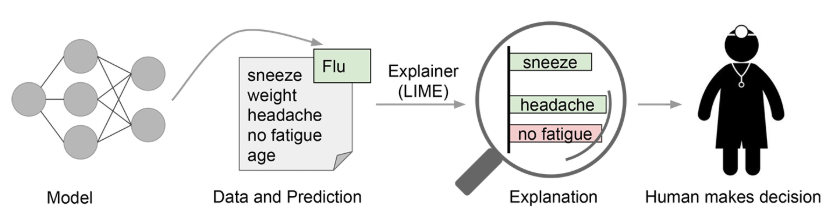
[Source: https://arxiv.org/abs/1602.04938]

#### 3.1.2 The idea behind LIME: The idea is quite intuitive. First, forget about the training data and imagine you only have the black box model where you can input data points and get the predictions of the model. You can probe the box as often as you want. Your goal is to understand why the machine learning model made a certain prediction. LIME tests what happens to the predictions when you give variations of your data into the machine learning model. LIME generates a new dataset consisting of permuted samples and the corresponding predictions of the black box model. On this new dataset LIME then trains an interpretable model, which is weighted by the proximity of the sampled instances to the instance of interest. The interpretable model can be anything from the interpretable models chapter, for example Lasso or a decision tree. The learned model should be a good approximation of the machine learning model predictions locally, but it does not have to be a good global approximation. This kind of accuracy is also called local fidelity. Mathematically, LIME interpretability constraint can be expressed as follows: $$\text{explanation}(x)=\arg <!--\; \; -->\underset{g\in <!--\; \in \; -->}{min}$$

  </mrow>
  <mi>G</mi>
</mrow>

L ( f , g , π x ) + Ω ( g )

The explanation model for instance x is the model g (e.g. linear regression model) that minimizes loss L (e.g. mean squared error), which measures how close the explanation is to the prediction of the original model $f$ (e.g. an random forest model), while the model complexity $\mathrm{\Omega <!--\; \Omega \; -->}(g)$ is kept low (e.g. prefer fewer features). G is the family of possible explanations, for example all possible linear regression models. The proximity measure ${\mathrm{\pi <!--\; \pi \; -->}}_x$ defines how large the neighborhood around instance x is that we consider for the explanation. In practice, LIME only optimizes the loss part. The user has to determine the complexity, e.g. by selecting the maximum number of features that the linear regression model may use.

The recipe for training the interpretable model:

• Select your instance of interest for which you want to have an explanation of its black box prediction.
• Perturb your dataset and get the black box predictions for these new points.
• Weight the new samples according to their proximity to the instance of interest.
• Train a weighted, interpretable model on the dataset with the variations.
• Explain the prediction by interpreting the local model.
  

In the current implementations in R and Python, for example, linear regression can be chosen as interpretable surrogate model. In advance, you have to select K, the number of features you want to have in your interpretable model. The lower K, the easier it is to interpret the model. A higher K potentially produces models with higher fidelity. There are several methods for training models with exactly K features. A good choice is Lasso. A Lasso model with a high regularization parameter λ yields a model without any feature. By retraining the Lasso models with slowly decreasing λ, one after the other, the features get weight estimates that differ from zero. If there are K features in the model, you have reached the desired number of features. Other strategies are forward or backward selection of features. This means you either start with the full model (=containing all features) or with a model with only the intercept and then test which feature would bring the biggest improvement when added or removed, until a model with K features is reached.

How do you get the variations of the data? This depends on the type of data, which can be either text, image or tabular data. For text and images, the solution is to turn single words or super-pixels on or off. In the case of tabular data, LIME creates new samples by perturbing each feature individually, drawing from a normal distribution with mean and standard deviation taken from the feature.

3.1.3 LIME for Tabular Data

Tabular data is data that comes in tables, with each row representing an instance and each column a feature. LIME samples are not taken around the instance of interest, but from the training data’s mass centre, which is problematic. But it increases the probability that the result for some of the sample points predictions differ from the data point of interest and that LIME can learn at least some explanation.

It is best to visually explain how sampling and local model training works:

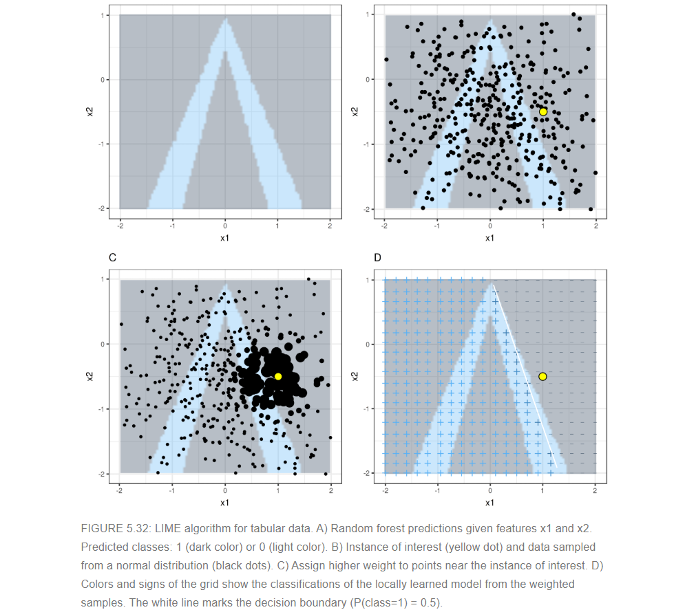
[Source: https://christophm.github.io/interpretable-ml-book/lime.html]

As always, the devil is in the detail. Defining a meaningful neighborhood around a point is difficult. LIME currently uses an exponential smoothing kernel to define the neighborhood. A smoothing kernel is a function that takes two data instances and returns a proximity measure. The kernel width determines how large the neighborhood is: A small kernel width means that an instance must be very close to influence the local model, a larger kernel width means that instances that are farther away also influence the model. If you look at LIME’s Python implementation (file lime/lime_tabular.py) you will see that it uses an exponential smoothing kernel (on the normalized data) and the kernel width is 0.75 times the square root of the number of columns of the training data. It looks like an innocent line of code, but it is like an elephant sitting in your living room next to the good porcelain you got from your grandparents. The big problem is that we do not have a good way to find the best kernel or width. And where does the 0.75 even come from? In certain scenarios, you can easily turn your explanation around by changing the kernel width.

3.1.4 LIME in application:

We demonstrate how LIME works in Python by working on real life application, we are going to use the “Loan dataset” from Kaggle, which can be found (here).

Dataset Problem Statement:

Our dataset is about “Dream Housing Finance” company, which deals in all home loans. They have presence across all urban, semi urban and rural areas. Customer first apply for home loan after that the company validates the customer eligibility for loan. The Company wants to automate the loan eligibility process (real time) based on customer detail provided while filling online application form. These details are Gender, Marital Status, Education, Number of Dependents, Income, Loan Amount, Credit History and others. To automate this process, they have given a problem to identify the customers segments, those are eligible for loan amount so that they can specifically target these customers.

First we take a glimpse at our data distribution

We train three classifiers and we train them on or data, predicting the target variable Loan_Status. we get the following accuracies:

Now we are going to explain

In the above code we build three classifiers and their LIME explainers, below we present the results for explaining the specified observation in the code above, where the first explanation blow is for the specified observation in the logistic regression classifier, the second explanation is for the same observation in random forest and the last one is for MLP classifier:

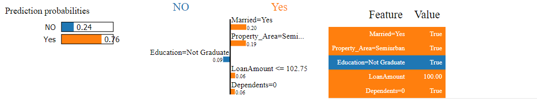
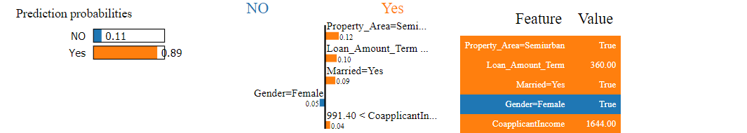
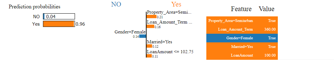
what can we actually see in the above results? we see the all our classifiers are having high probability for predicting Yes for giving a loan. The common most important features for predicting Yes for a loan in all my classifiers are Married perople and the people who are applying for a loan in the Semiurban area. We can say that the married yes feature got this importance because are represented in the training data twice more that single people as we saw in the data insight part, but we can make a statement about the semiurban people who got a really high importance in all classifiersieres even the Property-area features with almost evenly distributed. The gender female is getting importance as feature for predicting No for loan, but again almost 90 of the gender in our train where Man.

3.1.5 SP-LIME:

Although an explanation of a single prediction provides some understanding into the reliability of the classifier to the user, it is not sufficient to evaluate and assess trust in the model as a whole. So in the paper of Marco Tulio Riberio, Sameer Singh, and Carlos Guestrin [13] they provide another approach by extending their idea of LIME for explaining single observation and provide a global solution, they call that submodular pick. The approach is still model agnostic, and is complementary to computing summary statistics such as held-out accuracy.

3.1.6 How does SP-LIME works:

Lets demonstrate how submodular pick works by an example from the same paper [13]. In the below figure Rows represent instances (documents) and columns represent features (words)

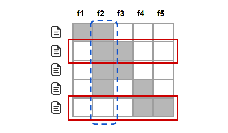
The first step it selects the number of instances, from the figure above we have five instances, second step it gets the explanation for each instance and we get the important features (in this case our important feature is f2 because it is relevant in four instances out of five), last step it picks the explanation with the highest coverage(rows two and five (in red) would be selected by the pick procedure, covering all but feature f1)

Now we apply the SP-LIME on our dataset and we see the results:

now looking at our global explanation for the code above we can answer our dataset problem statement, which was which area show the company consecrate on their marketing campaign and the answer is clearly the semiurban area which is the most important feature in our classifiers for getting a loan

3.2. Global Explanator Individual Conditional Exception plots (ICE)

Individual Conditional Exception plots or short ICE plots tackle the model inspection problem for any black box models by visualizing the estimated conditional expectations curves between a subset of predictors against the remaining predictor set. Alex Goldstein et al. [14] approach relies on Friedman’s work on partial dependence plots (PDP). Actually, one can describe ICE plots as disaggregated PDP plots. A PDP plots the change in the average partial relationship between two sets of predictors, one set varies over its marginal distribution. We also could ask: How a subset of predictors influencing the black box, if the remaining predictors stay equal?
A classical PDP plot visualizes one line for the change of the average partial relationship between the observed subset of predictors and the impact on the model behavior. However, ICE draws one line for each observation in the given dataset representing the individual impact of the observed predictor on the model predictions. We also can call these relationships as estimated conditional expectations curves. Hence ICE enables plotting of more complex interactions between predictions and predictors by highlighting the variation in the values across a covariate.
Below we will introduce PDP plots in general and then extend them to ICE plots. We will explain how to interpret the plots and give a practical demonstration with Scikit learn and code from scratch. Our black box models, a random forest and a neuronal network from Scikit, are trained with the loan data set from Kaggle. Finally, we close this chapter with an introduction of centered ICE (c-ICE) and derived ICE (d-ICE) plots.

3.2.1 PDP - Partial dependence plots

Partial dependence plots PDP) provide the basis for ICE plots. This approach visualizes the change of the average predicted value of a prediction model, when a subset of predictors varies over their marginal distribution. [14] In other words we take a dataset, preferably the training set of the black box model, combine each value of the observed predictors with each observation of the set and average the predictions of the black box model for this set.

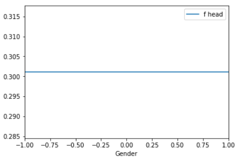
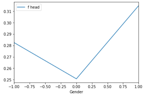
The PDPs above show the change in the average predicted value for the feature Gender on our neuronal network (left) and random forest (right). Zero represents a male and one a female applicant. A record with minus one represents an unknown gender. A flat line indicates a no impact on the observed features on the black box model. By comparing the PDPs above we can recognize that there is no impact of gender on the random forest (right). The neuronal network reacts stronger on the feature gender. A female applicant induced a higher change in the predicted values as a male one. But how we can compute a PDP?
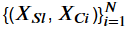
Before discussing the relying equitation, we want to make some assumptions and definitions. A training data set is defined as an amount of $N$ tuples, which contain a vector consisting of predictors ($X_i$) and a prediction ($Y_i$). A tuple is equal to one observation in the data set. The black box model ($\hat{f}$) maps the predictors ($X_i$,$p$) of an unknown number of observations to predictions ( $\hat{f}\left(X\right)$ ).

We assume that there exist two subsets of predictors. One is called $X_S$ and contains a certain number of predictors, which we want to test. The remaining predictors are collected in $X_C$ . $X_C$ and $X_S$ are complement sets to each other. Thus, we can formally define a PDP as follow.

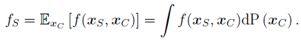
For creating a PDP we need to define a partial dependence function, which computes the average value of $f$ for a special $X_S$ and a $X_C$ which varies over its marginal distribution $dp\left(X_C\right)$. Each subset $X_S$ owns a partial dependence function. Unfortunately $f$ and $dp\left(X_C\right)$ are unknown. Furthermore we need another computable term.
We compute for each value in $X_S$ :

$X_{Ci}$represents a certain predictor tuple of the $X_C$ subset in the trainings data without the predictors of $X_S$. By using $\hat{f}$ instead of $f$ we are able to estimate the true model $f$ and by averaging over the observations in $X_C$ we estimate the integral over $X_C$. $N$ represents the number of observations in the training data set.
After computing the term above we get tuples like this one:

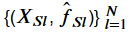
The tuple represents the estimated partial dependence function (${\hat{f}}_{Sl}$) at the $l$’th coordinate of $X_S$. By plotting and connecting of the tuples one creates the partial dependence plot (PDP). After this theoretical part we want to show how to implement a PDP function.
The main idea is to code a function, which iterates over the unique values of our $X_S$ set and replaces in each loop the observed features with one instance of the $X_S$ set. Then we store the result in a pandas data frame consisting two columns for the average predicted value and the corresponding $X_S$ value.

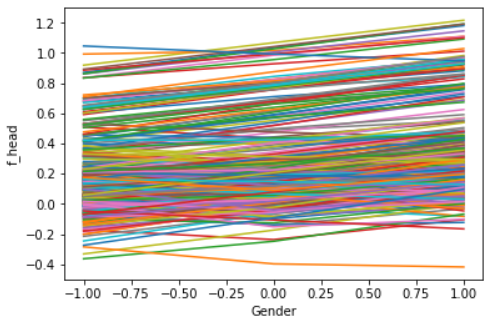
3.2.2 ICE - Individual Conditional Exception plots

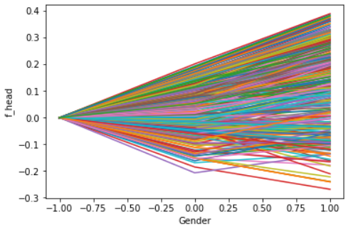
After introducing PDPs we will explain next Individual Conditional Exception plots (ICE) by Alex Goldstein et al. as an extension of PDP. An ICE can be described as a disaggregated PDP meaning that an ICE plots the estimated conditional expections curves for each prediction in the data set and not just the average. The curves refer to the functions of the prediction and the covariate $X_S$ relying on the an observed $X_C$.
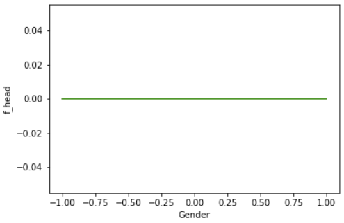
The left plot shows an ICE generated on the feature gender and our neuronal network. The left one is applied on the random forest model. We can easily recognize that most observations do not behave in the way the PDP plots above suggest. One can group the curves in the left plot in three groups. The first group increases from left to right. The second group decreases and the last one behaves like the PDP above shifted on the $y$ axis. The right plot shows shifted curves in the same way shaped. This indicates that the observed variable has no impact on the predictions of the model.

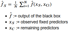
In the context of ICE observations are defined as a collection of tuples containing $X_S$ and the remaining predictors. The estimated response function is represented by $\hat{f}$. For each of the $N$ observations of $X_{Ci}$a line ${\hat{f}}_S^{\left(i\right)}$ is plotted against the observed values of $X_S$. This line defines the conditional relationship between $X_S$ and $\hat{f}$ at a certain point of $X_C$. As for PDP each value of $X_S$ is fixed while the $X_C$ varies across the observations. One can compute the ICE with the following algorithm:

The main idea is to iterate over the observations, fix one $X_C$ value per iteration and vary over the $X_S$ values. By visualizing the collected sets one can analyze how the observations behave if a certain feature differs. The code below computes the ICE for one black box model, a certain predictor $X_S$ and data set.

3.2.3 Colored ICE

What if want to know which features influence the behavior between our observed feature ($X_S$) and the predicted values? We could color lines depending on another feature. Below we plot an ICE for our random forest model depending on the feature Loan Amount with the Python package Pycebox. By coloring the second plot by education we can recognize that applicants with a brighter line get higher predicted values then darker ones.

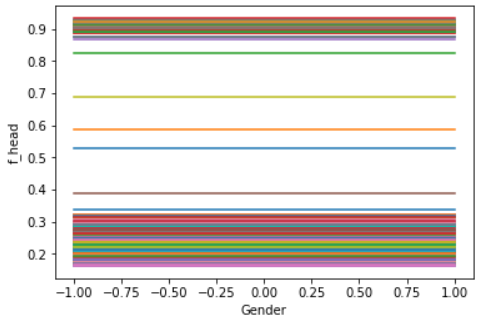
#### 3.2.4 Centered ICE plot (c-ICE) A centered ICE plot allows to visualize special effects, like “the variation in effects between curves and cumulative effects are veiled “([14], s. 5). By joining all curves at a certain coordinate ($X^{\backslash *}$) in $X_S$ an ICE removes level effects. The authors recommend the minimum or maximum value as $X^{\backslash *}$. If $X^{\backslash *}$ is the minimum, each curve will start at $0$ on the $y$ axis. Hence at the end of each curve represents the cumulative effect of $X_S$ on $\hat{f}$ relative to the base case ($X^{\backslash *}$).
The given c-ICE plots below show the same example as above. The right one visualizes the influence of gender on our random forest. All curves are stacked and flat, so we can assume that there are no changes on the predicted value at all. A c-ICE allows us easier to recognize the changes in an ICE. If we have a look on the left plot, we can determine taht the neuronal network reacts more sensitive on the gender of the applicant. Some observations just increase, decrease or behave like the PDP above.

The following function shows how to plot a c-ICE based on the output of our ICE function.

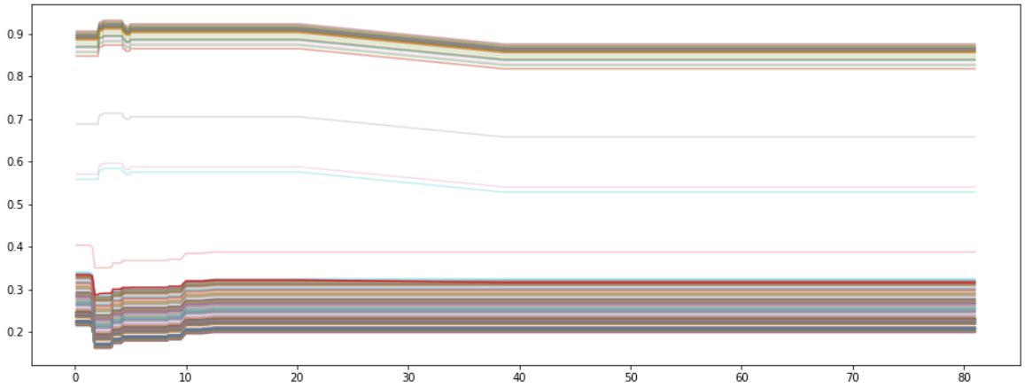
3.2.5 Derivate ICE plot

The derivate ICE (d-ICE) plot allows to explore interaction effects meaning that a relationship between $X_S$ and $\hat{f}$ relies on $X_C$. If no interaction between $X_S$ and $X_C$ exist, a normal ICE would plot several lines sharing an identical shape and shifted horizontal. D-ICE plots identical lines looking like a single line for no interaction between the predictors, and various lines for interaction.
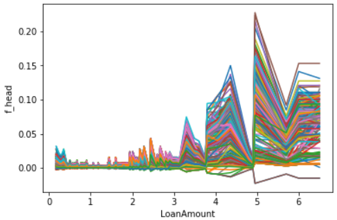
Our gender example with the random forest is a good example for d-ICE, that shows no interaction effects. In the d-ICE for the feature Loan Amount based on out neuronal network we can recognize that there are several areas of interaction, meaning that our variable Loan Amount depends on the remaining features.

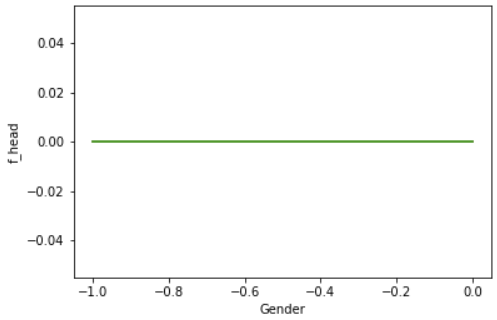
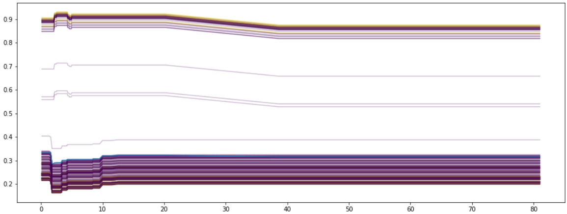
Goldstein et al. provided the algorithm below to compute the d-ICE. It only differs in line seven from the original ICE algorithm. Instead of using the raw prediction value, one first use Friedman’s Super Smoother and then computes the numerical partial derivative at the predictions.

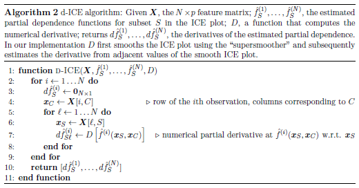
Our code computes the only the numerical partial derivative while plotting the d-ICE. We did not find a useable implementation of Friedman’s Super Smoother for Python.

4. Closing remarks

What we wanted to convey to the reader of this blog is, that it is very important to have the ability to explaining a black-box-system. The reader should see that is partly difficult to handle, a transparency of 100% is not possible, that an explanation can be interpreted differently and that this is the focus of ongoing research. We hope that our examples were interesting and gave a possibility for self-use. We think that this discussed issue for the blog will be a key discussion for the future, and we can be very excited to see how this all will develop in the next years.

References

[1] - EU Publication - General Data Protection Regulation- https://eur-lex.europa.eu/eli/reg/2016/679/oj

[2] - Goodman, B., & Flaxman, S. (2016). European Union regulations on algorithmic decision-making and a “right to explanation”. arXiv preprint arXiv:1606.08813.

[3] - press announcement – Website of the Federal Ministry for Economic Affairs and Energy https://www.bmwi.de/Redaktion/DE/Pressemitteilungen/2018/20181116-bundesregierung-beschliesst-strategie-kuenstliche-intelligenz.html

[4] - Guidotti, R., Monreale, A., Ruggieri, S., Turini, F., Giannotti, F., & Pedreschi, D. (2018). A survey of methods for explaining black box models. ACM Computing Surveys (CSUR), 51(5), 93.

[5] - Pedreschi, D., Giannotti, F., Guidotti, R., Monreale, A., Pappalardo, L., Ruggieri, S., & Turini, F. (2018). Open the Black Box Data-Driven Explanation of Black Box Decision Systems. arXiv preprint arXiv:1806.09936.

[6] - Lahav, O., Mastronarde, N., & van der Schaar, M. (2018). What is Interpretable? Using Machine Learning to Design Interpretable Decision-Support Systems. arXiv preprint arXiv:1811.10799.

[7] - Lipton, Z. C. (2016). The mythos of model interpretability. arXiv preprint arXiv:1606.03490.

[8] - Schneider, J., Handali, J. P., & vom Brocke, J. (2018, June). Increasing Trust in (Big) Data Analytics. In International Conference on Advanced Information Systems Engineering (pp. 70-84). Springer, Cham.

[9] - Zhou, Y., & Hooker, G. (2016). Interpreting Models via Single Tree Approximation. arXiv preprint arXiv:1610.09036.

[10] - Cortez, P., & Embrechts, M. J. (2013). Using sensitivity analysis and visualization techniques to open black box data mining models. Information Sciences, 225, 1-17.

[11] - Sensitivity Analysis Library in Python (Numpy) https://github.com/SALib/SALib

[12] - Fong, R. C., & Vedaldi, A. (2017). Interpretable explanations of black boxes by meaningful perturbation. arXiv preprint arXiv:1704.03296.

[13] – Ribeiro, Marco Tulio, Sameer Singh, and Carlos Guestrin. “Why Should I Trust You?: Explaining the predictions of any classifier.” Proceedings of the 22nd ACM SIGKDD international conference on knowledge discovery and data mining

[14] – Goldstein, A., Kapelner, A., Bleich, J.,& Pitkin, E. (2014). Peeking Inside the Black Box: Visualizing Statistical Learning with Plots of Individual Conditional Expectation. arXiv preprint arXiv: 1309.6392.

Appendix- Data Preparation ICE