By Andrew McAllister, Ivana Naydenova, Quang Nguyen Duc | February 8, 2019
 [Source:
 The task: Building a books recommendation engine 
Latent Dirichlet Allocation is a type of unobserved learning algorithm in which topics are inferred from a dictionary of text corpora whose structures are not known (are latent). The practical use of such an algorithm is to solve the cold-start problem, whereby analytics can be done on texts to derive similarities in the dictionary's corpses, and further be expanded to others outside the original scope - all without user input, which is often an early stumbling block for businesses that do not meet early usage quotas to derive needed analysis.
What we will be applying this to towards the end of this article is a recommendation engine for books based on their Wikipedia articles. Our recommendation engine aims to help users find books which might be interesting for them based on their summaries. At this point the algorithm is fully content based, lacking user input for collaborative filtering completely, but serves to illustrate the potential of such algorithms in forming the basis of high-level business implementable hybrid filters.
The data for the project - all books on Wikipedia - is collected from Wikipedia Dumps from the 1st of January, 2019, in their compressed forms. Using techniques outlined by Will Koehrsen of Medium's Towards Data Science we use a process of XML handlers to separate out individual pages, myparserfromhell's Wikipedia parser to derive the article titles, article contents, and length of each article, and further paralyze the process to assure optimal speed when going through all 15.8 GBs of compressed data (Link to the original article). Our thanks to Mr. Koehrsen for his techniques on how to access and create such an interesting data set for our analysis.
What follows is an overview of the related work on this topic followed by an explanation of the theoretics behind LDA to set the groundwork of our implementation. At the end, we will work through the full codes and present specific results of the algorithm, as well as discuss some of its shortcomings.
Related work 
The Latent Dirichlet Allocation (LDA) model and the Variational EM algorithm used for training the model were proposed by Blei, Ng and Jordan in 2003 (Blei et al., 2003a). Blei et al. (2003b) described LDA as a “generative probabilistic model of a corpus which idea is that the documents are represented as weighted relevancy vectors over latent topics, where a distribution over words characterizes a topic”. This topic model belongs to the family of hierarchical Bayesian models of a corpus, which has the purpose to expose the main themes of a corpus that can be used to classify, search, and investigate the documents of the corpus. In LDA models, a topic is a distribution over the feature space of the corpus, and several topics with different weights can represent each document. According to Blei et al. (2003a), the number of topics (clusters) and the proportion of vocabulary that create each topic (the number of words in a cluster) are considered to be tbe two hidden variables of the model. The conditional distribution of words in topics, given these variables for an observed set of documents, is regarded as the primary challenge of the model.
Griffiths and Steyvers (2004), used a derivation of the Gibbs sampling algorithm for learning LDA models to analyze abstracts from PNAS by using Bayesian model selection to set the number of topics. They proved that the extracted topics capture essential structure in the data, and are further compatible with the class designations provided by the authors of the articles. They drew further applications of this analysis, including identifying ‘‘hot topics’’ by examining temporal dynamics and tagging abstracts to illustrate semantic content. The work of Griffiths and Steyvers (2004) proved the Gibbs sampling algorithm is more efficient than other LDA training methods (e.g., Variational EM). The efficiency of the Gibbs sampling algorithm for inference in a variety of models that extend LDA is associated with the "the conjugacy between the Dirichlet distribution and the multinomial likelihood". Thus, when one does sampling, the posterior sampling becomes easier, because the posterior distribution is the same as the prior, and it makes inference feasible. Therefore, when we are doing sampling, the posterior sampling becomes easier. (Blei et al., 2009; McCallum et al., 2005).
Mimno et al. (2012) introduced a hybrid algorithm for Bayesian topic modeling, in which the main effort is to merge the efficiency of sparse Gibbs sampling with the scalability of online stochastic inference. Their approach decreases the bias of variational inference and can be generalized by many Bayesian hidden-variable models.
LDA is being applied in various Natural Language Processing tasks such as for opinion analysis (Zhao et al., 2010), for native language identification (Jojo et al., 2011) and for learning word classes (Chrupala, 2011).
In this blog post, we focus on the task of automatic text classification into a set of topics using LDA, in order to help users find books which might be interesting for them based on their summaries.
What is LDA? 
Latent Dirichlet Allocation is a type of unobserved learning algorithm in which topics are inferred from a dictionary of text corpora whose structures are not known (are latent). The practical use of such an algorithm is to solve the cold-start problem, whereby analytics can be done on texts to derive similarities in the dictionary's corpses, and further be expanded to others outside the original scope - all without user input, which is often an early stumbling block for businesses that do not meet early usage quotas to derive needed analysis.
What we will be applying this to towards the end of this article is a recommendation engine for books based on their Wikipedia articles. Our recommendation engine aims to help users find books which might be interesting for them based on their summaries. At this point the algorithm is fully content based, lacking user input for collaborative filtering completely, but serves to illustrate the potential of such algorithms in forming the basis of high-level business implementable hybrid filters.
The data for the project - all books on Wikipedia - is collected from Wikipedia Dumps from the 1st of January, 2019, in their compressed forms. Using techniques outlined by Will Koehrsen of Medium's Towards Data Science we use a process of XML handlers to separate out individual pages, myparserfromhell's Wikipedia parser to derive the article titles, article contents, and length of each article, and further paralyze the process to assure optimal speed when going through all 15.8 GBs of compressed data (Link to the original article). Our thanks to Mr. Koehrsen for his techniques on how to access and create such an interesting data set for our analysis.
What follows is an overview of the related work on this topic followed by an explanation of the theoretics behind LDA to set the groundwork of our implementation. At the end, we will work through the full codes and present specific results of the algorithm, as well as discuss some of its shortcomings.
In order to understand the kind of books that a certain user likes to read, we used a natural language processing technique called Latent Dirichlet Allocation (LDA )used for identifying hidden topics of documents based on the co-occurrence of words collected from those documents.
The general idea of LDA is that
each document is generated from a mixture of topics and each of those topics is a mixture of words.
Having this in mind, one could create a mechanism for generating new documents, i.e. we know the topics a priori, or for inferring topics present in a set of documents which is already known for us. This bayesian topic modelling technique can be used to find out how high the share of a certain document devoted to a particular topic is, which allows the recommendation system to categorize a book topic, for instance, as 30% thriller and 20% politics. These topics will not and do not have to be explicitly defined. Managers looking to apply LDA will often expect that outputs of specific topic classes will be provided by the analysis, but this is often extraneous - or potentially harmful to the robust potential of the analysis when a topic set is chosen such that they can be easily defined by human intuition. In our analysis, we will directly name any of our found topics, but will draw the reader's attention to when the words do seem to fit in a potential topic.
Concerning the model name, one can think of it as follows (Blei et al., 2003a):
Latent: Topic structures in a document are latent meaning they are hidden structures in the text.
Dirichlet: The Dirichlet distribution determines the mixture proportions of the topics in the documents and the words in each topic.
Allocation: Allocation of words to a given topic.
Parameter estimation 
LDA is a generative probabilistic model, so to understand exactly how it works one needs first to understand the underlying probability distributions. The idea behind probabilistic modeling is (Blei et al., 2003a):
- to treat data as observations that arise from some kind of generative probabilistic process (the hidden variables reflect the thematic structure of the documents (books) collection),
- to infer the hidden structure using posterior inference (What are the topics that describe this collection?) and
- to situate new data into the estimated model (How does a new document fit into the estimated topic structure?)
In the next sectios we will focus on the multinomial and Dirichlet distributions utilized by LDA.
Inference 
Having specified the statistical model structure, the crucial part now is to find a method for estimating the relevant parameters. As shown in the previous section, our model is based on the joint probability distribution over both observable data and hidden model parameters. Such models are considered as probabilistic generative models. In comparison, discriminative models like e.g. logistic regression or SVMs, directly model the conditional probability $P(Y|X=x)$ of some target variable $Y$ with given observations $x$.
Parameter estimation, or more precisely statistical inference, on generative models are generally approached by Bayesien inference. In essence, bayesian inference applies the Bayes theorem on statistical models to draw conclusions from the data about the parameter distribution of interest.
Bayes Theorem 
Before introducing the concept of Baysian inference, it is necessary to provide the Bayes' theorem. An advantage of this theorem is the ability to include prior knowledge or belief to calculate the probability of related events.
Mathematically, the Bayes' theorem can be stated as follows: $$P(A|B)=\frac{P(B|A)P(A)}{P(B)}$$ where
- $A$ and $B$ are events with $P(B)\neq0$
Model-Based Bayesian Inference 
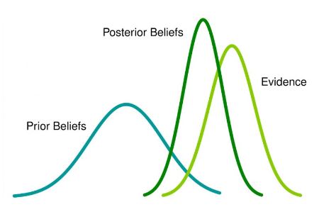
The introductory definition of Bayes' rule will now be adopted to the model form in order to represent the data and parameters. In the section above we have only used single numbers for the terms in the Bayes' theorem equation. However, when applying Bayes' rule to more complex machine learning models, this is not sufficient. As prior beliefs often contain uncertainty, probability distributions over a range of values are more appropriate. The same logic applies to the other terms of the equation. Therefore, probabilities $P(.)$ are replaced by densities $p(.)$.
Furthermore, the events $A$ and $B$ are replaced by the model parameters and the observed data. The observed data is represented by $y=\{y_1,y_2,...,y_N\}$ and the set of parameters (which we are typically interested in) is denoted as $\Theta$ Taking everything into account and using the Bayes' rule, the Baysian inference model is formalized as
$$p(\Theta|y)= \frac{p(y|\Theta)p(\Theta)}{p(y)}$$
with the following components:
- $p(\Theta)$ is the prior distribution (or simply: prior) of the parameter set $\Theta$ and is used as a means of expressing uncertainty about $\theta$ before observing the data. As a probability distribution, it contains its own set of parameters which are called hyperparameters, to differentiate them from the model parameters $\Theta$.
- $p(y|\Theta)$ is the sampling distribution, which models the probability of observable data $y$ given latent model parameters $\Theta$. It is also often called the likelihood (function) when it is viewed as a function of $\Theta$.
- $p(y)$ defines the marginal likelihood of $y$ and is also called the evidence.
- $p(\Theta|y)$ is the posterior distribution giving the updated probability of the parameters $\Theta$ after taken both the prior and the data into account
Multinomial Distribution 
Instead of maximum-likelihood, Bayesian inference encourages the use of predictive densities and evidence scores. This is illustrated in the context of the multinomial distribution, where predictive estimates are often used but rarely described as Bayesian (Minka, 2003).
Now we will describe the multinomial distribution which is used to model the probability of words in a document. For this reason, we will also discuss the conjugate prior for the multinomial distribution, the Dirichlet distribution.
Given a set of documents, one can choose values for the parameters of a probabilistic model that make the training documents have high probability (Elkan, 2014). Considering a test document, one can evaluate its probability according to the model: The higher the probability is, the more similar the test document is to the initial set of documents. For this purpose, the multinomial distribution could be applied with the following probability distribution function:
$$ p(x; \theta)=\bigg(\frac{n!}{\prod^{m}_{j=1}}\bigg)\bigg(\prod^{m}_{j=1}\theta_{j}^{x_{j}}\bigg), $$ where $\theta_{j}$ is the probability of word j while $x_{j}$ is the count of a word j.
So every time, a certain word j appears in the document it contributes an amount $\theta_{j}$ to the total
probability ( $\theta_{j}^{x_{j}}$).
In this equation, the first factor in parentheses is called a multinomial coefficient, which represents the size of the equivalence class of x, while the second factor in parentheses is the probability of any individual member of the equivalence class of x.
Dirichlet distribution — what is it, and why is it useful? 
The Dirichlet distribution is used for representation of the distributions over the simplex (the set of N-vectors whose components sum to 1) and is a useful prior distribution on discrete probability distributions over categorical variables.
It is a conjugate prior to the categorical and multinomial distributions (meaning that multiplying a Dirichlet prior by a multinomial or categorical likelihood will yield another Dirichlet distribution of a certain form). However, the primary difference between Dirichlet and multinomial distributions is that Dirichlet random variables are real-valued, where each element of the vector is in the interval $[0, 1]$, and multinomial random variables are integer-valued.
The Dirichlet distribution defines a probability density for a vector valued input having the same characteristics as our multinomial parameter $\theta$.
\begin{equation} Dir (\vec\theta\mid \vec\alpha)={\frac {\Gamma (\Sigma_{i=1}^{K}\alpha_{i})}{\prod _{i=1}^{K}\Gamma (\alpha_{i})}}\prod _{i=1}^{K}\theta_{i}^{\alpha_{i}-1} \end{equation}
This equation is often represented using the Beta function in place of the first term as seen below:
\begin{equation} Dir (\vec\theta\mid \vec\alpha)={\frac {1}{B(\alpha)}}\prod _{i=1}^{K}\theta_{i}^{\alpha_{i}-1} \end{equation}
Where:
\begin{equation} \frac {1}{B(\alpha)} = {\frac {\Gamma (\Sigma_{i=1}^{K}\alpha_{i})}{\prod _{i=1}^{K}\Gamma (\alpha_{i})}} \end{equation}
The Dirichlet distribution is parameterized by the vector $\alpha$, which has the same number of elements K as our multinomial parameter $\theta$ (Thomas Boggs, 2014). Thus, one could interpret $p(\theta \mid\alpha)$ as responding to the question “what is the probability density associated with multinomial distribution $\theta$, given that our Dirichlet distribution has parameter $\alpha$.
To get a better sense of what the distributions look like, let us visualize a few examples in the context of topic modeling.
The Dirichlet distribution takes a number ($\alpha$) for each topic. The GIF below shows the iterations of taking 1000 samples from a Dirichlet distribution using an increasing alpha value. Every topic gets the same alpha value one could see displayed, and the dots represent a distribution or mixture of the three topics having certain coordinates such as (0.6, 0.0, 0.4) or (0.4, 0.3, 0.3). Low $\alpha$-values account for the case where most of the topic distribution samples are in the corners (near the topics). Having values (1.0, 0.0, 0.0), (0.0, 1.0, 0.0), or (0.0, 0.0, 1.0) would mean that the observed document would only ever have one topic in case a three topic probabilistic topic model is build.
Usually, one aims to end up with a sample favoring only one topic or a sample that gives a mixture of all topics, or something in between. In case the $\alpha$-values>1, the samples start to congregate to the center. With greater $\alpha$ the samples will more likely be uniform or a homogeneous mixture of all the topics.
Typically one aims to find more than three topics depending on the number of observed documents. In the ideal case, the composites to be made up of only a few topics and our parts to belong to only some of the topics.
from IPython.display import Image
from IPython.core.display import HTML
Image(url= "https://cdn-images-1.medium.com/max/800/1*_NdnljMqi8L2_lAYwH3JDQ.gif", width=700)
LDA as a Generative process 
LDA is being often described as the simplest topic model (Blei and Lafferty, 2009): The intuition behind this model is that documents exhibit multiple topics. Furthermore, one could most easily describe the model by its generative process by which the model assumes the documents in the collection arose (Blei, 2012).
LDA can be described more formally with the following notation:
 [Source: Blei, 2012.]
- A document-to-topic model parameter $\theta_{m}$ is used to generate the topic for the $n^{th}$ word in the doument d denoted by $z_{m,n}$, for all n of [1; N].
- A topic-to-word model $\phi_{k}$ is used to generate the word $w_{m,n}$ for each topic $k=z_{m,n}$
Those two steps can be seen on the graphical model above, where the document-to-topic model and the topic-to-word model essentially follow multinomial distributions (counts of each topic in a document or each word in a topic), a good prior for their parameters, would be Dirichlet distribution, explained here.
Assuming that the word distributions for each topic vary based on a Dirichlet distribution, as do the topic distribution for each document, and the document length is drawn from a Poisson distribution, one can generate the words in a two-stage process for each document in the whole data collection:
- Randomly choose a distribution over topics.
For each word in the document:
- A topic is being randomly chosen from the distribution over topics in the first step.
- Sample parameters for document topic distribution
- $\theta_{m}$ follows the $Dir(\alpha_{m}\mid \alpha)$ distribution, after observing topics in the document and obtaining the counting result $n_{m}$, one could calculate the posterior for $\theta_{m}$ as $Dir(\alpha_{m}\mid n_{m}+\alpha)$. Thus, the topic distribution for the mth document is $$ p(z_{m}\mid \alpha)=\frac{\Delta(n_{m}+\alpha)}{\Delta(\alpha)} $$ and the topic distribution for the all document is
$$ p(z\mid\alpha)= p(w,z\mid\alpha,\beta)= \displaystyle\prod_{m=1}^{M}\frac{\Delta(n_{m}+\alpha)}{\Delta{\alpha}} $$
we assume, similarly, for the kth topic, that the prior for the topic-to-word model's parameter $\phi_k$ follows the $Dir(\phi_k\mid \beta)$ distribution, after observing words in the topic and obtaining the counting result $n_{k}$, one could calculate the posterior for $\phi_{k}$ as $Dir(\phi_k\mid n_{k}+\beta)$. Thus, the word distribution for the kth topic is
$$ p(w_{k}\mid z_{k}, \beta)=\frac{\Delta(n_{k}+\beta)}{\Delta(\beta)} $$ and the word distribution for the all topics is
$$ p(w_{k}\mid z, \beta)=\displaystyle\prod_{m=1}^{M}\frac{\Delta(n_{k}+\beta)}{\Delta(\beta)} $$
- A topic is being randomly chosen from the distribution over topics in the first step.
The distinctive characteristic of LDA is that all the documents in the collection share the same set of topics and each document exhibits those topics in different proportion.
Using this notation, the generative process for LDA is equivalent to the following joint distribution of the hidden and observed variables (Blei, 2012):
\begin{equation*} p(w,z\mid\alpha,\beta)=p(w\mid z,\beta)p(z\mid \alpha)=\displaystyle\prod_{k=1}^{K}\frac{\Delta(n_{k}+\beta)}{\Delta{\beta}}\displaystyle\prod_{m=1}^{M}\frac{\Delta(n_{m}+\alpha)}{\Delta{\alpha}} \end{equation*}
Posterior computation for LDA 
As already mentioned,
the aim of topic modelling is to automatically discover the topics from a collection of documents, which are observed, while the topic structure is hidden.
This can be thought of as “reversing” the generative process by asking what is the hidden structure that likely generated the observed collection?
We now turn to the computational problem, computing the conditional distribution of the topic structure given the observed documents (called the posterior.) Using our notation, the posterior is
$$p(\theta,\phi, z \mid w, \alpha, \beta) = \frac{p(\theta,\phi, z, w, \mid \alpha, \beta)}{p(w, \mid \alpha, \beta)}$$
The left side of the equation gives us the probability of the document topic distribution, the word distribution of each topic, and the topic labels given all words (in all documents) and the hyperparameters $\alpha$ and $\beta$. In particular, we are interested in estimating the probability of topic (z) for a given word (w) (and our prior assumptions, i.e. hyperparameters) for all words and topics.
A central research goal of modern probabilistic modelling is to develop efficient methods for approximating the posterior inference (Blei, 2012).
Gibbs sampling 
The general Idea of the Inference process is the following (Tufts, 2019):
- Initialization: Randomly select a topic for each word in each document from a multinomial distribution.
- Gibbs Sampling:
- For i iterations
- For document d in documents:
- For each word in document d:
- assign a topic to the current word based on probability of the topic given the topic of all other words (except the current word).
- For each word in document d:
This procedure is repeated until the samples begin to converge to what would be sampled from the actual distribution. While convergence is theoretically guaranteed with Gibbs Sampling, there is no way of knowing how many iterations are required to reach the stationary distribution (Darling, 2011). Usually, an acceptable estimation of convergence can be obtained by calculating the log-likelihood or even, in some situations, by inspection of the posteriors.
When applying LDA, one is interested in the latent document-topic portions $\theta_{d}$, the topic-word distributions $\phi(z)$, and the topic index assignments for each word $z_{i}$. While conditional distributions – and therefore an LDA Gibbs Sampling algorithm – can be derived for each of these latent variables, we note that both $\theta_{d}$ and $\phi(z)$ can be calculated using just the topic index assignments $z_{i}$ (Darling, 2011). To this reason, Griffiths and Steyvers (2004) applied a simpler algorithm, called collapsed Gibbs sampler, which integrates out the multinomial parameters and sample $z_{i}$.
To compute the collapsed Gibbs sampler updates efficiently, the algorithm maintains and makes use of several count matrices during sampling (Papanikolaou et al., 2017):
- $n_{kv}$ represents the number of times that word type v is assigned to topic k across the corpus,
- $n_{dk}$ represents the number of word tokens in document d that have been assigned to topic k.
The equation giving the probability of setting $z_{i}$ to topic k, conditional on $w_{i},d$, the hyperparameters $\alpha$ and $\beta$, and the current topic assignments of all other word tokens (represented by ·) is:
$$p(z_{i}=k\mid w_{i}=v, d, \alpha, \beta, ·)\propto \frac{n_{kv\neg i}+\beta_{v}}{\Sigma_{v'=1}^{V}(n_{kv\neg i}+\beta_{v})} . \frac{n_{dk\neg i}+\alpha_{k}}{N_{d}+\Sigma_{k'=1}^{K}\alpha_{k'}}$$
The exclusion of the current topic assignment of $w_{i}$ of from all count matrices is annotated by $\neg i $. A common practice is to run the Gibbs sampler for many iterations before retrieving estimates for the parameters, and the one can retrieve estimates for the variables of interest.
By using Rao-Blackwell estimators Griffiths and Steyvers, (2004) computed a point estimate of the probability of word type v given topic k ($\hat{\phi_{kv}}$) and a point estimate for the probability of the topic k given document d ($\hat{\theta_{dk}}$):
$$ \hat{\phi_{kv}}=\frac{n_{kv}+\beta_{v}}{\Sigma_{v'=1}^{V}(n_{kv}+\beta_{v})} $$
$$ \hat{\theta_{dk}}=\frac{n_{dk}+\alpha_{k}}{N_{d}+\Sigma_{k'=1}^{K}\alpha_{k'}} $$
When applying the collapsed Gibbs sampler on new documents during the prediction stage, a common practice is to fix the $\phi$ distributions and set them to the ones learned during estimation:
$$p(z_{i}=k\mid w_{i}=v, d, \alpha,\hat{\phi_{kv}} , ·)\propto \hat{\phi_{kv}} . \frac{n_{dk\neg i}+\alpha_{k}}{N_{d}+\Sigma_{k'=1}^{K}\alpha_{k'}}$$
Variational Inference 
Blei et al. (2003) first introduced LDA using an inference method based on variational inference. As the derivation and its mathematical details are out of scope for this introduction to the LDA, we provide an intuition for the steps involved. The general idea of this method is to approximate the intractable posterior distribution $P$ by a tractable distribution $Q_V$ with a set of free variational parameters $V$. The goal then is to eventually find parameters $V$ which minimizes the Kullback-Leibler (KL) divergence $KL(Q_V||P)=\sum Q_V \log{\frac{Q_V}{P}}$. The key advantage is that this process can be done without computing the actual posterior distribution and still approach the posterior up to an constant, which is independent of the variational parameters. Moreover, these parameters $V$ are only dependend on the obervable data $w$.
Model
The specific approach taken here is referred as a mean field approximation, where we assume the following:
- All target variables are independent of each other
- Each variable has its own variational parameter
With these assumptions, we can set up the model:
- Probability of topic $z$ given document $d$: $q(\theta_d|\gamma_d)$
Each document has its own Dirichlet prior $\gamma_d$ - Probability of topic assignment to word $w_{d,n}$: $q(z_{d,n}|\phi_{d,n})$
Each $n^{th}$-word in document $d$ has its own multinomial over topics $\phi_{d,n}$
Inference
The inferential step estimates the parameters of $q(\theta,z|\gamma,\phi)$ by minimizing the KL divergence
$$KL[q(\theta,z|\gamma,\phi) \ || \ p(\theta,z|w,\alpha,\beta)]$$
The KL divergence, also known as relative entropy, is a function which quantitatively measures the "difference" between two probability distributions. Thus, the lower the value of KL, the more similar are both distributions $q(\theta,z|\gamma,\phi)$ and $p(\theta,z|w,\alpha,\beta)$. The optimization problem is therefore given by
$$\gamma^*,\phi^* = argmin_{(\gamma,\phi)} KL[q(\theta,z|\gamma,\phi) \ || \ p(\theta,z|w,\alpha,\beta)]$$
Using the definition of the KL divergence function, Blei et. al (2003) derive the equation
$$KL[q(\theta,z|\gamma,\phi) \ || \ p(\theta,z|w,\alpha,\beta)] = - L(\gamma, \phi|\alpha,\beta) + \log p(w, \alpha,\beta)$$
with $L(\gamma, \phi|\alpha,\beta) = E_q[\log p(\theta, z, w|\alpha,\beta)]-E_q[\log q(\theta,z|\gamma, \phi)]$
and additionally applying Jensen's inequality, it follows the inequality
$$\log p(w|\alpha, \beta) \geq L(\gamma, \phi|\alpha,\beta)$$
In the first equation we can see that the minimization problem turns into a maximization problem of some likelihood function $L(\gamma, \phi|\alpha,\beta)$, as the second term is constant and can be ignored. The left hand side of the second equation shows the log-likelihood of the evidence of our posterior distribution. This inequality is commonly knows as the evidence lower bound, abbreviated as ELBO. The interpretation of this ELBO has some positive insights: As we aim to maximize $L(\gamma, \phi|\alpha,\beta)$ (which is equivalent to minimize the KL divergence), we simultaneously maximize the lower bound of our evidence. Remember that the evidence gives the probability of our observed data, given our model parameters. Hence, by optimizing the parameters, we increase our confidence of the observed data. In fact, this is similar to the intuition of the maximum likelihood estimation, where we estimate parameters such that the probability of our observed data is maximum. What we can see on the left hand side is the log-likelihood of the evidence of our posterior probability, whereas $L(\gamma, \phi|\alpha,\beta)$ represents the equivalent optimzation
Variational EM-algorithm
However, a closed-form solution can not be derived for maximizing the objective function $L(\gamma, \phi|\alpha,\beta)$. Hence, Blei et. al have proposed a variational expectation maximization (variational EM) algorithm to iteratively solve this optimization problem.
The derivation of the parameter estimatiosn by using the variational EM algorithm is quite lengthy but the intuition can be summarized as follows:
Goal: Find $\alpha, \beta$ which maximize the marginal log-likelihood $l(\alpha,\beta|w)=\sum_d \log p(w_d|\alpha,\beta)
- Define and initialize a tractable distribution $q(\theta,z|\gamma,\phi)$ that defines a lower bound of the log-likelihood of the actual data.
- Iterate the two following steps until $l(\alpha,\beta|w)$ converges:
- E-step: Update $\gamma^*, \phi^*$ to get new approximated posteriors $q(\theta,z|\gamma,\phi)$. For each document, find optimal values of its variational parameters. This is basically the optimization equation above.
- M-step: Update $\alpha, \beta$ to get new evidence $p(\theta, z, w|\alpha,\beta)$. The parameters $\alpha, \beta$ are chosen such that the resulting lower bound of the log likelihood are maximum. Usually this corresponds to finding maximum likelihood estimates of $\alpha, \beta$ for each document under the new approximate posterior $q(\theta,z|\gamma^*,\phi^*)$
Book Similarity Computation 
LDA and Jaccard Similarity 
As already mentioned, we will apply the LDA algorithm to extract the latent topics within Wikipedia's book summaries. This is followed by aggregation of most frequently occurring topics and their utilization in order to calculate the Jaccard Similarity between the topics of other book summaries. The combination of latent topics and similarity measurement allows one to uncover both topics and apparent relationships between the summaries of two establishments (Yang and Provinciali, 2015).
The Jaccard similarity coefficient measures similarity between two finite sample sets A and B by counting the number of items they have in common and dividing by the total number of unique items between them:
\begin{equation*} J(A,B)= \frac{\mid A \cap B \mid}{\mid A \cup B\mid } \end{equation*}
When the Jaccard similarity coefficient is above a certain threshold, a high correlation between the latent characteristics of two books is implied.
However, a content-based recommendation system will not perform on the highest level, if there is no data on user’s preferences, regardless of how detailed our metadata is.
Implementation - an LDA Recommendation Engine for Books 
Let's start by uploading the base Python packages, as well as tools to remove expressions from the texts, pickle to save us some time, plotting packages, and json to load the data.
import os
import pandas as pd
import numpy as np
import datetime as dt
import time

%load_ext ipycache

import random
import re
import pickle

import matplotlib.pyplot as plt
import seaborn as sns

import json

from IPython.core.display import display, HTML
display(HTML("<style>.container { width:99% !important; }</style>"))
project_folder = os.getcwd()
Loading the Data
We begin by loading the book data that we derived from the January 1st 2019 Wikipedia dumps, removing those with 'Wikipedia:' in their name, as these are pages for Wikipedia contributors (see below). To start, we have 37,523 books. This total number will be reduced, and the total words within each corpus will be further reduced after tokenization.
books = []

with open(project_folder+'/wiki/found_books_filtered.ndjson', 'r') as fin:
    books = [json.loads(l) for l in fin]

books_with_wikipedia = [book for book in books if 'Wikipedia:' in book[0]]
books = [book for book in books if 'Wikipedia:' not in book[0]]
print(f'Found a total of {len(books)} books.')
As stated before, each book entry contains the title, the text of the article (not necessarily including the title in the first part), the date of last edit (unused), and a rough estimate of how long the article is in charachters.
Data Exploration and Preparation
To begin our data exploration, let's derive first what data types we're dealing with.
print('List of Books type: {}'.format(type(books)))
print('Book type: {}'.format(type(books[0])))
print('Title type: {}'.format(type(books[0][0])))
print('Text type: {}'.format(type(books[0][1])))
print('Edit date type: {}'.format(type(books[0][2])))
print('Length type: {}'.format(type(books[0][3])))
Now let's look at some elements of each book list element - first the titles, then the descriptions, and then the lengths.
for i in range(5):
    print(books[i][0])
print(books[0][1])
for i in range(5):
    print(books[i][3])
The maximum and minimum article lengths should be found to set basic bounds to reduce our articles corpus based on unsuitible lengths.
def max_article_length(books_list):
    return max([books_list[x][3] for x in range(len(books_list))])

def min_article_length(books_list):
    return min([books_list[x][3] for x in range(len(books_list))])

print('Maximum article text length is: {}'.format(max_article_length(books)))
print('Minimum article text length is: {}'.format(min_article_length(books)))
Let's now find which books have the longest and shortest article lengths. Cache the data after the first run to avoid running it again.
%%cache mycache_article_lengths.pkl longest_article, shortest_article
longest_article = None
shortest_article = None

# Longest and shortest book articles:
for i in range(len(books)):
    if books[i][3] == max_article_length(books):
        longest_article = [books[i][0], books[i][3]]

for i in range(len(books)):
    if books[i][3] == min_article_length(books):
        shortest_article = [books[i][0], books[i][3]]
print(longest_article)
print(shortest_article)
Removing Books
The following defines a function that removes a book from the list based on indexes that we will derive. The list object that is the book will be replaced by the string 'Delete me!', and all entries that are not this string will be kept. In looking at the titles of the books collected, those that had a semicolon were shown to be those that were most likely not singular books, so I focused on that to remove unneeded articles.
def book_remover(books_list, removal_index_list):
    for i in removal_index_list:
        books_list[i] = 'Delete me!'
    books_list = [book for book in books_list if book != 'Delete me!']
    return books_list
We use book remover to delete the following kinds of articles:
- Commentaries
- Dr. Who Anthologies
- Draft Articles
- Lists of Books
- Anthologies
- Short Story Collections
Deriving Most Popular Books
For further exploration of the corpus, let's look into which book titles appear most often in the article texts of other books. Again pickling the results, as this cell takes a very long time to run.
%%cache mycache_title_frequencies.pkl title_frequencies

def title_freq_generator(books_list):
    title_frequencies = []
    prog_marker = 0
    for i in range(len(books_list)):
        freq = 0
        book = books_list[i]
        title = book[0]
        other_book_indexes = list(range(len(books_list)))
        other_book_indexes.remove(i)
        for o in other_book_indexes:
            if title in books_list[o][1]:
                freq += 1
        title_frequencies.append((title, freq))
        prog_marker += 1

        if prog_marker % 1000 == 0:
            print('{} title frequencies have been found.'.format(prog_marker))
    return title_frequencies

title_frequencies = title_freq_generator(books)
What's the result?
most_frequent_mentions = sorted(title_frequencies, key=lambda x: x[1], reverse=True)
most_frequent_mentions[25:50]
We used the above range to remove common English word books that appear at the top. Some famous books that appeard before place 25 were: The Road by Cormac McCarthy, The Trial (Der Process) by Franz Kafka, Encyclopedia Britannica, The Encyclopedia of Science Fiction, Dracula by Bram Stoker, and The Prince by Niccolò Machiavelli. The novels obviously benefited from having relatively common names, which is to say nothing of their content. Furthermore, the obvious omission is The Bible, which is does not have a book infobox, and is thus not a part of the dataset.
The encyclopedias would thus rank first and second, and Cervantes gets the award for the most mentioned novel on English Wikipedia with Don Quixote. May Don Quixote and Sancho Panza be ever appreciated for their battles against ferocious giants that are actually windmills.
Cleaning Book Names
Now that we've done an analysis of titles in text bodies, let's remove the parethases from them. This was not done before this step so as to avoid further common English words from being added to the frequency aggregation. Famous books rarely have (novel) or (book).
for i in range(15):
    print(books[i][0])

def book_tag_remover(books_new, books_old):
    for x in range(len(books_old)):
        books_old[x][0] = re.sub(r'\(.*?\)', '', books_old[x][0])
        if books_old[x][0][-1] == ' ': # Removes the space that's left at the end of the books that have the tag removed
            books_old[x][0] = books_old[x][0][:-1]
        books_new.append(books_old[x])

    return books_new
books_no_tag = []

print('-----')
books_no_tag = book_tag_remover(books_no_tag, books)
for i in range(15):
    print(books_no_tag[i][0])
Dealing With the Article Length Distribution
And now we proceed further with some necessary cleaning. Let's look at the distribution of article lengths that we have.
def roundup_100(x):
    return x if x % 100 == 0 else x + 100 - x % 100

def round_lengths(books_list):
    return [roundup_100(books_list[x][3]) for x in range(len(books_list))]

rounded_to_100_lengths = round_lengths(books_no_tag)
print(rounded_to_100_lengths[:5])
length_counts = {x:rounded_to_100_lengths.count(x) for x in rounded_to_100_lengths}
print(sorted(length_counts.items())[:5])

x = [tup[0] for tup in sorted(length_counts.items())]
y = [tup[1] for tup in sorted(length_counts.items())]

plt.figure(figsize=(20,10))
plt.bar(x,y, width=100)
plt.title('Number of Articles by Article Length', fontsize=30)
plt.xlabel("Ranges of Article Lengths (by 100 charaters)", fontsize=20)
plt.ylabel("Number of Articles", fontsize=20)
plt.show()

As we can see, there is an inordinate number of books with almost no length, and that is matched by books at the higher end of the spectrum that upon inspection are shown to have large sections on cultural significance.
The shortest articles were found to simply be those that said that an author wrote a book, with nothing else in its content.
And now the longest books should be inspected.
longest_articles = books_sorted[round(len(books_sorted)*0.9995):]

# Longest books:
for i in range(len(longest_articles)):
    print(longest_articles[i][0])
Obviously we do not need the books at the short end of the article length spectrum. LDA is not going to assign meaningful topics when the only words to derive topics from are the author's name, year or release, and the collection it appears in - even more so when considering that some words may be removed later post tokenization, where some of these words may be removed because they're stop words, appear to frequently, or aren't long enough.
We'll thus remove those books in the bottom 20% of article length and the last three books in the catalogue, which are all collections. Ultimately the decision to not remove a percentage of books at the end of the distribution was made to keep certain extremely influential books in the greater text corpus.
books_no_stub = books_sorted[round(len(books_sorted)*0.20):len(books_sorted)-3]
print('Number deleted: {} | Current catalogue: {} books'.format(len(books_sorted) - len(books_no_stub), len(books_no_stub)))
Let's look again and what we have for the length distribution, and note that we will be dealing with the longer articles in another way once the texts have been tokenized.
rounded_to_100_lengths = round_lengths(books_no_stub)

length_counts = {x:rounded_to_100_lengths.count(x) for x in rounded_to_100_lengths}
print(sorted(length_counts.items())[:5])

x = [tup[0] for tup in sorted(length_counts.items())]
y = [tup[1] for tup in sorted(length_counts.items())]

plt.figure(figsize=(20,10))
plt.bar(x,y, width=100)
plt.title('Number of Articles by Article Length', fontsize=30)
plt.xlabel("Ranges of Article Lengths (by 100 charaters)", fontsize=20)
plt.ylabel("Number of Articles", fontsize=20)
plt.show()

Final Text Cleanup
Before we switch over to the tokenized articles, we should switch all articles to one line bodies, remove real expression references, remove those parts of the text that are used to distinguish between parts of an article, remove possessives, remove websites, and finally reduce all spaces in the articles to single spaces such that post cleaning we'll have a readable body.
def text_one_liner(books_list):
    for x in range(len(books_list)):
        books_list[x][1] = books_list[x][1].replace('\n', ' ')
    return books_list

books_clean = text_one_liner(books_no_stub)
def real_exp_remover(books_list):
    for x in range(len(books_list)):
        books_list[x][1] = re.sub(r'\<.*?\>', '', books_list[x][1])
        books_list[x][1] = re.sub(r'\[.*?\]', '', books_list[x][1])
    return books_list

books_clean = real_exp_remover(books_clean)
unneeded_filler = ['Category:', '(hardcover)', '(paperback)', '==External links==', '==Consequences==', '==Discussion==',
                   '==References==', '==Plot==', '==Contents==', '==Reception==', '==Notes==', '==Themes==', '==Miniseries adaptation==',
                   '==Sources==', '==See also==', '==Plot summary==', '==Quotations==', '==Publication==',
                   '==Title==', '== References ==', '== External links ==', '==Further reading==', '==Introduction==',
                   '==Main characters==', '==Release details==', '===Summary===', '*', '====', '===', '==', '& nbsp;', '.com', 'jpg', '❤']

def filler_remover(books_list):
    for x in range(len(books_list)):
        for filler in unneeded_filler:
            books_list[x][1] = books_list[x][1].replace(filler, '')
    return books_list

books_clean = filler_remover(books_clean)
def possessive_fixer(books_list):
    for x in range(len(books_list)):
        books_list[x][1] = books_list[x][1].replace("\'", "")
    return books_list

books_clean = possessive_fixer(books_clean)
def website_remover(books_list):
    for x in range(len(books_list)):
        websites = []
        for word in books_list[x][1].split(' '):
            if word[:4] == 'http':
                websites.append(word)

        for website in websites:
            books_list[x][1] = books_list[x][1].replace(website, '')
    return books_list

books_clean = website_remover(books_clean)
def space_reducer(books_list):
    for x in range(len(books_list)):
        for i in range(25, 0, -1): #Loop backwards to assure that smaller spaces aren't made by larger deletions and then missed
            large_space = str(i*' ')
            if large_space in books_list[x][1]:
                books_list[x][1] = books_list[x][1].replace(large_space, ' ')
    return books_list

books_clean = space_reducer(books_clean)
books_clean[0]
Preparing Articles for Data Analysis
The following was done to prepare articles for dataanalysis:
- The book articles are removed from the initial list of book properties
- Punctuation is removed
- Article strings are turned into tokens, and stop words are removed
- Numeric tokens were removed
- Bigrams are created
- Words are lemmatized to reduce words of similar roots to similar tokens
- English first names are removed, as these are often very prevalent in articles (note that bigrams of full names are retained)
- Token amounts per article are rounded off at an exponentially increasing rate (we'll more explain when we get there)
- Tokens of that are less than four characters are removed
- Only tokens that appear in at least ten articles are kept
- Those tokens that appear in more than 15% of all articles will be removed
And here we are to the stage where we need to get rid of the extra information at the end of articles. To do this, we looked at the longest book article in our text corpus - Finnigan's Wake (article here: https://en.wikipedia.org/wiki/Finnegans_Wake). The sections slowly decrease in topic modeling importance starting with "Allusions to Other Works," which would help us connect it to other novels via bigrams, and its Norwegian influences, leading to the section on 100 letter words that Joyce uses.
The hundred letter words, for example:
bababadalgharaghtakamminarronnkonnbronntonnerronntuonnthunntrovarrhounawnskawntoohoohoordenenthurnuk
... were all deleted when the real expressions were removed from the text. In the section though the word "hundredlettered" appears, which appears only once in the text. We'll use this as our reference point for where we want the text to be shortened. Let's first find at what point this word is found.
articles_no_name[-1].index('hundredlettered')
articles_no_name[-1].index('hundredlettered')/len(articles_no_name[-1])
Let's further look at our distribution of tokens per article.
def round_lengths_exp(articles_list):
    return [roundup_100(len(articles_list[x])) for x in range(len(articles_list))]
rounded_to_100_now = round_lengths_exp(articles_no_name)

length_counts_now = {x:rounded_to_100_now.count(x) for x in rounded_to_100_now}
print(sorted(length_counts_now.items())[:20])

x_now = [tup[0] for tup in sorted(length_counts_now.items())]
y_now = [tup[1] for tup in sorted(length_counts_now.items())]

plt.figure(figsize=(20,10))
plt.bar(x_now, y_now, width=100)
plt.title('Current Number of Articles by Token Amount', fontsize=30)
plt.xlabel("Ranges of Token Amounts (by 100)", fontsize=20)
plt.ylabel("Number of Articles", fontsize=20)
plt.show()

Our goal is thus to write a function to remove the last 30% of the Finnegans Wake article and other similarly long articles, but remove little or no words from smaller articles. We'll achive this by using the fact that our articles are ordered by length, and write an exponential funciton. We'll count up by index in the list of books as we go through it, and put this value into a sixth degree polynomial such that the rate of increase will be rapid.
To prevent it from increasing in the early part of the article distribution, we'll multiply the funciton by a very small decimal to keep all initial values close to 0 until such a time when the exponential increase is fast enough to overcome the initial reduction. Looking at the table above, with roughly half of our articles having less than 400 tokens, and then the amounts drastically increase, let's design a function that's close to 0 until 15,000, and then increases rapidly to around 0.3 at our maximum article index of 29543.
x_vals = list(range(len(articles_no_name)))
x_vals[:5]
length = len(x_vals)
print(length)

y_vals = [0.00000000000000000000000000045*(x**(6)) for x in x_vals]
y_vals[:5]
plt.figure(figsize=(10,5))
plt.plot(x_vals, y_vals, linestyle='solid')

Trial and error at its finest. The y-values of the above function will thus be the amounts rouded off of the end of each article, or more specifically 1 minus these amounts will be multiplied by the length of the token amount per article and used as the upper bound for token subsetting, with the lower bound of course being 0.
import math

def remove_last(new_list, old_list):
    prog_marker = 0
    for article in old_list:
        article_percent_remaining = 1-(0.00000000000000000000000000045*(prog_marker**(6)))
        new_article = article[:round(len(article)*article_percent_remaining)]
        new_list.append(new_article)
        prog_marker += 1

#         if prog_marker % 1000 == 0:
#             print('{} articles have had their sizes reduced.'.format(prog_marker))

    print(token_counter(new_list, old_list))

    return new_list
articles_last = []

articles_last = remove_last(articles_last, articles_no_name)
print(articles_last[0])
Let's take a look at our new distribution.
rounded_to_100_new = round_lengths_exp(articles_last)

length_counts_new = {x:rounded_to_100_new.count(x) for x in rounded_to_100_new}
print(sorted(length_counts_new.items())[:20])

x_new = [tup[0] for tup in sorted(length_counts_new.items())]
y_new = [tup[1] for tup in sorted(length_counts_new.items())]

plt.figure(figsize=(20,10))
plt.bar(x_new, y_new, width=100)
plt.title('New Number of Articles by Token Amount', fontsize=30)
plt.xlabel("Ranges of Token Amounts (by 100)", fontsize=20)
plt.ylabel("Number of Articles", fontsize=20)
plt.show()

Our upper bound has decreased by 30%, and the early articles were unaffected. It does seem to cluster the articles at the tail a bit more than in the original graph, but let's not split hairs over whether a seventh or eigth degree polynomial with an even more restrictive initial divisor would be more appropriate.
We continue now to short tokens. As stated before, tokens under four characters are removed.
From here we continue with the other cleaning processes that can be found in the main notebook.
Let's see what the most common words in our text corpus are!
text_word_frequency = Counter(chain.from_iterable(articles_model))
text_word_frequency.most_common()[:15]
Model Prep
We've already imported our LDA package gensim for its Phrases tool within its models, and now we'll import the rest of the parts we'll need.
from gensim import corpora, models, similarities
First, let's create our dictionary, which is a mapping between the words in our corpus and their integer representations. The cell after next will display a few examples of the mappings.
%%time

dictionary = corpora.Dictionary(articles_model)
from itertools import islice
def take(n, iterable):
    return list(islice(iterable, n))

items_5 = take(5, dictionary.iteritems())
items_5
Now we convert our documents into bag of words (BoW) format, where each will be represented by tuples of token id and token count.
%%time

bow_corpus = [dictionary.doc2bow(text) for text in articles_model]
How many tokens and articles do we have?
print('Number of unique tokens: %d' % len(dictionary)) # roughly 400 less than in presentation
print('Number of articles: %d' % len(bow_corpus)) # roughly 500 less than in presentation
And what does The Great Sea: A Human History of the Mediterranean look like now?
print(bow_corpus[0])
def tokenization_report(bow, article_number):
    article_tokens = bow[article_number]
    sorted_tokens = sorted(article_tokens, key=lambda x: x[1], reverse=True)
    for i in range(len(bow[article_number])):
        print("Word {} (\"{}\") appears {} time(s).".format(sorted_tokens[i][0],
                                                         dictionary[sorted_tokens[i][0]],
                                                         sorted_tokens[i][1]))
tokenization_report(bow_corpus, 0)
We can see from the above words that it will be quite difficult to come up with an accurate prediction for the above book. We'll find that with books tht have more specific tokens that link them to similar books, that the results are more obvious, but there is a lot of noise above. There are the languages at the end, that it references countless European countries - so we're hoping it would be referred to other books that are a summary of a European region and are "critically acclaimed history that chronicles civilization" - to use other tokens.
Determining Optimal Topic Number
At this point we need to determine our optimal number of topics. We do this as we would using cluthering methods like k-nearest neighbors, by producing models at a regularly increasing interval of topic amounts, and using an elbow method based on the Jaccard similarity to select an amount that gives sufficient coverage, but doesn't over cover such that the topics are overly similar and incldue too many articles.
For the upcoming LDA model, we'll need to understand the following:
- num_topics: number of requested latent topics to be extracted from the training corpus.
- passes: number of passes through the corpus during training.
- update_every: number of documents to be iterated through for each update. 1 = iterative learning.
And of course, we'll be using random state 42. What respectable programming project on books would not use 42 as is practice - in homage to the Hitchhiker's Guide to the Galaxy. It is "The Answer to the Ultimate Question of Life, The Universe, and Everything."
topicnums = [1,5,10,15,20,25,30,35,40,45,50]
project_folder = os.getcwd()

ldamodels_bow = {}
for i in topicnums:
    random.seed(42)
    if not os.path.exists(project_folder+'/models/ldamodels_bow_'+str(i)+'.lda'):
        %time ldamodels_bow[i] = models.LdaModel(bow_corpus, num_topics=i, random_state=42, update_every=1, passes=10, id2word=dictionary)
        ldamodels_bow[i].save(project_folder+'/models/ldamodels_bow_'+str(i)+'.lda')
        print('ldamodels_bow_{}.lda created.'.format(i))
    else:
        print('ldamodels_bow_{}.lda already exists.'.format(i))
lda_topics = {}
for i in topicnums:
    lda_model = models.LdaModel.load(project_folder+'/models/ldamodels_bow_'+str(i)+'.lda')
    lda_topics_string = lda_model.show_topics(i)
    lda_topics[i] = ["".join([c if c.isalpha() else " " for c in topic[1]]).split() for topic in lda_topics_string]

pickle.dump(lda_topics,open(project_folder+'/models/pub_lda_bow_topics.pkl','wb'))
Now that we have our models, we need to find what the best number of topics is. As stated before, we'll be using Jaccard Similarity:
- A statistic used for comparing the similarity and diversity of sample sets.
- J(A,B) = (A ∩ B)/(A U B)
- Goal is low Jaccard scores for coverage of the diverse elements
We'll first define a function, then compute the Jaccard similarities accross the topics at each topic number level, and then graph these to find our elbow point.
def jaccard_similarity(query, document):
    intersection = set(query).intersection(set(document))
    union = set(query).union(set(document))
    return float(len(intersection))/float(len(union))
lda_stability = {}
for i in range(0,len(topicnums)-1):
    jacc_sims = []
    for t1,topic1 in enumerate(lda_topics[topicnums[i]]):
        sims = []
        for t2,topic2 in enumerate(lda_topics[topicnums[i+1]]):
            sims.append(jaccard_similarity(topic1,topic2))
        jacc_sims.append(sims)
    lda_stability[topicnums[i]] = jacc_sims

pickle.dump(lda_stability,open(project_folder+'/models/pub_lda_bow_stability.pkl','wb'))
lda_stability = pickle.load(open(project_folder+'/models/pub_lda_bow_stability.pkl','rb'))
mean_stability = [np.array(lda_stability[i]).mean() for i in topicnums[:-1]]

with sns.axes_style("darkgrid"):
    x = topicnums[:-1]
    y = mean_stability
    plt.figure(figsize=(20,10))
    plt.plot(x,y,label='Average Overlap Between Topics')
    plt.xlim([1, 55])
    plt.ylim([0, 0.25])
    plt.xlabel('Number of topics')
    plt.ylabel('Average Jaccard similarity')
    plt.title('Average Jaccard Similarity Between Topics')
    plt.legend()
    plt.show()

Deploying Optimal Model
From above we can see that the similarity continues to decrease after 30, and the decrease is farily consistent. We don't want too many topics, so we'll use that as our optimal model.
num_topics = 30
lda_model_final = models.LdaModel.load(project_folder+'/models/ldamodels_bow_'+str(num_topics)+'.lda')
Here's where it starts to get really good! Let's look at our topics. The next cell will print all 30 topics. Each entry will have the top 10 words by significance, followed by the whole topics coherence - the average of the pairwise word-similarity scores of all words within the topic.
from pprint import pprint
top_topics = lda_model_final.top_topics(bow_corpus, topn=10)

avg_topic_coherence = sum([t[1] for t in top_topics]) / num_topics
print('Average topic coherence: %.4f.' % avg_topic_coherence)

counter = 0
for topic in top_topics:
    print('Topic {}:'.format(counter))
    counter += 1
    pprint(topic)

pickle.dump(lda_topics,open(project_folder+'/models/pub_lda_bow_topics.pkl','wb'))
Again let's return to The Great Sea: A Human History of the Mediterranean. Of which topics is it composed?
corpus_lda_model = lda_model_final[bow_corpus]
for article in corpus_lda_model[0]:
    print(article)
It's highest correlated topic was 13, which is: game, dragon, player, rule, adventure, monster, class, master, spell, dungeon. Not the best, but with the others we should be able to get more influences to culture and the Mediterranean. (Full disclosure, there are countless books on Dungeons and Dragons in the Corpus that we couldn't fully eliminate, and they do have a tendency to muddy up the results, as seen in topic 13.)
Let's do one final check based on our articles being ordered by length. It would make sense that longer articles would be composed of more topics than shorter ones, so let's graph the topic correlation of the highest correlated optic for each article and see if we can a decreasing relation.
from operator import itemgetter
index_high_corr_list = []

index_counter = 0

for article in corpus_lda_model:
    highest_feature = max(article, key=itemgetter(1))[0]
    max_correlation = max(article, key=itemgetter(1))[1]
    index_high_corr_list.append([index_counter, highest_feature, max_correlation])
    index_counter += 1

index_high_corr_list[:5]
x = [tup[0] for tup in index_high_corr_list]
y = [tup[2] for tup in index_high_corr_list]

plt.figure(figsize=(20,10))
scatter = plt.plot(x,y, '.')
line = plt.plot(np.unique(x), np.poly1d(np.polyfit(x, y, 1))(np.unique(x)), 'r')
plt.title('Highest Correlation of Topics/Article Length', fontsize=30)
plt.xlabel("Article Length Rank Ordered", fontsize=20)
plt.ylabel("Highest Topic Correlation", fontsize=20)
plt.show(scatter, line)

Not quite as steep of a decline as we expected, but enough to confirm that we're on the right track (AKA haven't done anything too wrong).
Recommender Demonstration
We're now ready to make our recommendations! Just one final explanation of cosine similarity, which we will use to compare the vectors of assigned topics and their coherences per article.
- Cosine similarity measures between bag of words vectors give us similarities in the range of -1 to 1 (the greater, the more similar)
- Similarity = cos(θ) = (A‧B)/(‖A‖‖B‖), ‖X‖ being its norm
We order these outputs for recommendations based on a user chosen book. In the following cell we initialize the similarity matrix between all BoW articles, which we will order for querried books and use as the basis for our recommendations. Be sure to cache the following cell.
%%cache mycache_lda_index.pkl index

index = similarities.MatrixSimilarity(lda_model_final[bow_corpus])
And now for the recommender!
It has the following steps:
- A book title is entered by the user
- The matching book title is found in the corpus (or a similar one is suggested as before)
- The similarities of all orther books are quierried from index, our similarity matrix
- These similarities are enumerated such that a similarity score can be matched to the corresponding title
- The recommendation scores for all books are appended to a previously created empty list
- These recommendation scores are ordered
- The following is printed:
- The first ten most common tokens in the books article
- The main topic for the book
- The 2nd to 11th recommendations (first element would be the querried book itself)
def book_recommender(title):
    books_checked = 0
    for i in range(len(books_clean)):
        recommendation_scores = []
        if books_clean[i][0] == title:
            lda_vectors = corpus_lda_model[i]
            sims = index[lda_vectors]
            sims = list(enumerate(sims))
            for sim in sims:
                book_num = sim[0]
                recommendation_score = [books_clean[book_num][0], sim[1]]
                recommendation_scores.append(recommendation_score)

            recommendation = sorted(recommendation_scores, key=lambda x: x[1], reverse=True)
            print("Your book's most prominent tokens are:")
            article_tokens = bow_corpus[i]
            sorted_tokens = sorted(article_tokens, key=lambda x: x[1], reverse=True)
            sorted_tokens_10 = sorted_tokens[:10]
            for i in range(len(sorted_tokens_10)):
                print("Word {} (\"{}\") appears {} time(s).".format(sorted_tokens_10[i][0],
                                                             dictionary[sorted_tokens_10[i][0]],
                                                             sorted_tokens_10[i][1]))
            print('-----')
            print("Your book's most prominant topic is:")
            print(lda_model_final.print_topic(max(lda_vectors, key=lambda item: item[1])[0]))
            print('-----')
            print('Here are your recommendations for "{}":'.format(title))
            display(recommendation[1:11])

        else:
            books_checked +=1

        if books_checked == len(books_clean):
            book_suggestions = []
            print('Sorry, but it looks like "{}" is not available.'.format(title))
            other_books = []
            for x in range(len(books_clean)):
                other_book = books_clean[x][0]
                book_silimarity = round(similar_books(other_book, title), 2)
                similarity_score = [other_book, book_silimarity]
                book_suggestions.append(similarity_score)

            print('-----')
            ordered_suggestions = sorted(book_suggestions, key=lambda x: x[1], reverse=True)
            print('Were any of the following maybe what you were looking for?')
            print(ordered_suggestions[:10])
Now to check some books! The following list was made up to comprise a large span of different types of books including popular fantasy books like Harry Potter and the Lord of the Rings, to one of the most loved children's books, to James Bond for action and spy novels, to one of the pinacles of historical fiction, to a major work in science finction, and finishing with a work of philosophy that coincedentally has one of our longest articles. Each recommendation will be followed by a short discussion of the results.
Books to check:
- Harry Potter and the Philosopher's Stone
- The Fellowship of the Ring
- Where the Wild Things Are
- The Man with the Golden Gun
- Adventures of Huckleberry Finn
- Critique of Pure Reason
Harry Potter and the Philosopher's Stone
book_recommender("Harry Potter and the Philosopher's Stone")
Any Harry Potter book always come up with other books in the series, and in one case it came up with the other six, but this was a run where what could be considered a Harry Potter topic was made. We're missing the Prisoner of Azkaban. With the bigram harry_potter appearing so much, as well as rowling, hermione, and voldomort, you'd expect that the model would be able to consistently connect them all together, but these results are fine.
Let's take a quick look at the connection between the Philosopher's Stone and the Prisoner of Azkaban. For that, we'll need another function.
def book_comparer(title1, title2):
    books_checked = 0
    for i in range(len(books_clean)):
        similarity = []
        if books_clean[i][0] == title1:
            lda_vectors1 = corpus_lda_model[i]
            sims = index[lda_vectors1]
            for j in range(len(books_clean)):
                if books_clean[j][0] == title2:
                    lda_vectors2 = corpus_lda_model[j]
                    similarity.append(sims[j])
                    print('The similarity between {} and {} is: {}'.format(title1, title2, similarity[0]))

                    print('-----')
                    print("{}'s most prominent tokens are:".format(title1))
                    article_tokens = bow_corpus[i]
                    sorted_tokens = sorted(article_tokens, key=lambda x: x[1], reverse=True)
                    sorted_tokens_10 = sorted_tokens[:10]
                    for i in range(len(sorted_tokens_10)):
                        print("Word {} (\"{}\") appears {} time(s).".format(sorted_tokens_10[i][0],
                                                                     dictionary[sorted_tokens_10[i][0]],
                                                                     sorted_tokens_10[i][1]))

                    print('-----')
                    print("{}'s most prominant topic is:")
                    print(lda_model_final.print_topic(max(lda_vectors1, key=lambda item: item[1])[0]))

                    print('-----')
                    print("{}'s most prominent tokens are:".format(title2))
                    article_tokens = bow_corpus[j]
                    sorted_tokens = sorted(article_tokens, key=lambda x: x[1], reverse=True)
                    sorted_tokens_10 = sorted_tokens[:10]
                    for i in range(len(sorted_tokens_10)):
                        print("Word {} (\"{}\") appears {} time(s).".format(sorted_tokens_10[i][0],
                                                                     dictionary[sorted_tokens_10[i][0]],
                                                                     sorted_tokens_10[i][1]))

                    print('-----')
                    print("{}'s most prominant topic is:")
                    print(lda_model_final.print_topic(max(lda_vectors2, key=lambda item: item[1])[0]))
book_comparer("Harry Potter and the Philosopher's Stone", "Harry Potter and the Prisoner of Azkaban")
We were 1% off of having all six other Harry Potter books suggested. The disimilarity of the Prisoner of Azkaban is aparent though. The most frequent word is black - for Serius Black - which would strongly correlate to other books, and the bigram harry_potter appears half as much in prisoner as in the Philosopher's Stone. That they both still had the same main topic is promising as well.
The Fellowship of the Ring
book_recommender("The Fellowship of the Ring")
The Lord of the Rings is another positive yet problematic entry. As with Harry Potter, you get some, but sometimes not them all. For full disclosure, if you do the Return of the King, you just get the two Towers, but the first book of the series gives us not only the the other two, but also the prequil in the Silmarilion, and a book finished by Tolkein's son in the Children of Hurin. Other books seem random, or are of the fantasy genre. Maybe looking into a version of LDA that places higher importance on those tokens at the top of the frequency list would be a worthwhile endeavor. This is certainly the case for the next entry.
Interestingly, the Hobbit is in many ways unrelated to the Lord of the Rings, but often comes up with books by C.S. Lewis like The Lion, The Witch, and the Wardrobe. This is to a degree unsurprising, as Lewis and Tolkein were members of the Inlkings, a writing group at Oxford, and thus were highly influential on one another. Lewis is mentioned three times in the Hobbit's article.
Let's compare The Fellowship of the Ring and The Hobbit. First, here are the recommendations for the Hobbit.
book_recommender("The Hobbit")
As stated, the top two recommendations come from CS Lewis' The Chronicle's of Narnia. Beren and Lúthien is a book finished by Christopher Tolkein, and J. R. R. Tolkien's influences makes sense given the focus of the article on Tolkein's influences when writing the Hobbit.
book_comparer("The Fellowship of the Ring", "The Hobbit")
Again we have the same first topic, but the simiarity is 10% lower than our top 10 threshhold. Tolkein appears an astounding 75 times in the text for the Hobbit, as the author's first major work. Further, the topics of the Lord of the Rings and the Hobbit are distinct for LDA in ways that they might not be for us. The Hobbit has goblins and far more dwarves, the Lord of the Rings has orcs, and the felowship itself is an important token.
Where the Wild Things Are
book_recommender("Where the Wild Things Are")
Famous kids books are hard to predict, as their articles are often full of parts on cultural significance that may not have been entirely reduced. In this model, if we do say Charlotte's Web, then the results are chaotic. With Where the Wild Things Are we get all kids books, and beyond that many famous ones in Yertle the Turtle and The Polar Express.
What we didn't get was another book by the author, Maurice Sendak. Let's compare Where the Wild Things Are with In the Night Kitchen, another great book by him.
book_comparer("Where the Wild Things Are", "In the Night Kitchen")
What we see is that the content of the books is simply too different. They don't even have the same main topic. In the first we have a journey to a mysterious island with friendly monsters, and in the second we again have a journey, but this time to a kitchen where the main character bakes cakes. Sandek appears mutlipe times in each article, but not enough to make up for the overarching difference. This could only be solved if say the articles themselves were tagged by author in a process within the recommendation, but outside of LDA.
The Man with the Golden Gun
book_recommender("The Man with the Golden Gun")
The recommender is good at picking out James Bond books. Period. Every single one of those books is another James Bond book. It is rare that it doesn't come up with at least eight others in the top 10, but that's also because Flemming wrote 14, and in total there are over 50. Flemmings novels are thankfully those that are predicted, but when you have such a large portion of the corpus on one character, it's no surprise that it's easy to find other books about him.
Adventures of Huckleberry Finn
book_recommender("Adventures of Huckleberry Finn")
Adventures of Huckleberry Finn would be a very hard book to make recommendations for based on token content. There're so many topics in play. Getting Tom Sawyer is necessary, and that it's so high is a plus. The natural suggestion would be other classics of US-American literature, but that would require words that describe that to be more weighted than others. What we get instead is solcio-political commentary about the US, which makes sense, but getting major works like The Grapes of Wrath would be better.
Critique of Pure Reason
book_recommender("Critique of Pure Reason")
Critique of Pure Reason and all other major works of philosophy fare well with the analysis. This is also likely because there are so many "acceptable suggestions." The same can be said for conceptual science books.
With that being said, and to our credit, Critique of Pure Reason is the first of a trilogy, with the other two being found in the top three, and the top four all being by or about Kant. Further, the Ninth book is about Critique of Pure Reason, and the eigth book being Hegel's master work is another plus due to the influence of Kant on Hegel.
Overall:
- The model does a fairly good job of suggesting books in a series to others in the same series
- It does an ok good job at suggesting books by the same author that are not in a series
- It does a good job of making general genre suggestions
- The above suggestions though are not related to the cultural significance of the book, so relatively unkown books are still easily recommended
- It does a bad job on books that have significance beyond their base story
- It's hard to judge efficiency of books with short vs. long articles, as we frankly wouldn't know what the ones with short articles should be recommended in the first place. What we do note though is that such books are recommended to those with long articles where they are seen as not belonging
As a side note to one wanting to try this - pay very very careful attention to the final step of the cleaning. Dropping words that are in too many articles has a dramatic effect on the results based on the chosen threshhold. Ours is set at 15%, and both 10% and 20% had dramatically worse results - say only two Harry Potter Books, and almost random results for Where the Wild Things Are.
Graphically Representing Topics
import pyLDAvis.gensim
First and foremost, and heartfelt thanks to pyLDAvis for such an amazing package to allow us to really show the data and let it be manipulated to boot. The following graph is composed of two pannels:
The left panel, labeld Intertopic Distance Map: circles represent different topics, with the distance corresponding to their relative similarities. The relative frequency of the topic in the corpus is further represented by he size of a topic's circle. An individual topic may be selected for closer scrutiny by clicking on its circle, or entering its number in the "selected topic" box in the upper-left.
The right panel, the bar chart of the top 30 terms: when no topic is selected in the plot on the left, the bar chart shows the top-30 most saliant (footer 1) terms in the corpus. By saliant we mean not simply the frequency of said term in the corpus, but further its ability to distinguish between different topics. By selecting each topic on the left, one modifies the bar chart to show the relevant (footer 2) terms for the selected topic. Relevence can be tuned by parameter λ. A smaller λ gives higher weight to the term's distinctiveness, while a larger λ s corresponds to probablity of the term occurance per topics.
Further, the axes of the graph are two principle coordinates used in the multidimmensional scaling.
vis = pyLDAvis.gensim.prepare(lda_model_final, bow_corpus, dictionary)
pyLDAvis.display(vis)
Model Evaluation
One major way of elvaluating an LDA model is to split the texts in half and compare the topic assignment for each half. The more similar the topic assignment, the better.
from sklearn.metrics.pairwise import cosine_similarity
articles_model_1 = [article[:np.int0(len(article)/2)] for article in articles_model]
articles_model_2 = [article[np.int0(len(article)/2):] for article in articles_model]
We'll now transform the data as before, and use our model to create LDA corpuses.
corpus_1 = [dictionary.doc2bow(article) for article in articles_model_1]
corpus_2 = [dictionary.doc2bow(article) for article in articles_model_2]
lda_corpus_1 = lda_model_final[corpus_1]
lda_corpus_2 = lda_model_final[corpus_2]
The following function returns the topics with non-zero weight through a matrix tranformation of docs within the topic space.
from collections import OrderedDict
def article_topic_dist(model, corpus, kwords=False):
    top_dist =[]
    keys = []

    for d in corpus:
        tmp = {i:0 for i in range(num_topics)}
        tmp.update(dict(model[d]))
        vals = list(OrderedDict(tmp).values())
        top_dist += [np.array(vals)]
        if kwords:
            keys += [np.array(vals).argmax()]

    return np.array(top_dist), keys
top_dist_1, _ = article_topic_dist(lda_model_final, lda_corpus_1)
top_dist_2, _ = article_topic_dist(lda_model_final, lda_corpus_2)

print("Intra similarity: cosine similarity for corresponding parts of a doc(higher is better):")
print(np.mean([cosine_similarity(c1.reshape(1, -1), c2.reshape(1, -1))[0][0] for c1,c2 in zip(top_dist_1, top_dist_2)]))

random_pairs = np.random.randint(0, len(articles_model), size=(400, 2))

print("Inter similarity: cosine similarity between random parts (lower is better):")
print(np.mean([cosine_similarity(top_dist_1[i[0]].reshape(1, -1), top_dist_2[i[1]].reshape(1, -1)) for i in random_pairs]))
A 16% difference is well within what we saw as acceptable for differences between the similarity values - better than most - and that it comes with the upper bound at 87% is an added plus.
Recommending Based on Outside Text
The beauty of LDA is that it can easily be applied to texts outside the greater text corpus. All we need to do is tokenize the text, create a BoW representation of it using our dictionary, and then we'll again do a similarity querry against our corpus to get predictions as before.
First we'll define a new function to do a rough tokenization of any text we find on the internet, and then proceed with an example text. In this instance we'll be using the Wikipedia summary of Macbeth. Plays are sadly not categorized with the same infoboxes as books, so they were not included in the analysis. Something to consider adding in for future iterations.
def text_to_tokens(raw_text):
    clean_text = raw_text.lower()
    for ch in clean_text:
        for p in punctuation_exclude:
            if ch == p:
                clean_text = clean_text.replace(ch, ' ')
    tokens = [token for token in clean_text.split() if token not in stop_words]
    lemmed_tokens = [wordnet_lemmatizer.lemmatize(token) for token in tokens]
    lemmed_tokens = [wordnet_lemmatizer.lemmatize(token, pos='v') for token in lemmed_tokens]

    return [token for token in lemmed_tokens if len(token) > 3]
other_text = '''
Act I
The play opens amid thunder and lightning, and the Three Witches decide that their next meeting will be with Macbeth. In the following scene, a wounded sergeant reports to King Duncan of Scotland that his generals Macbeth, who is the Thane of Glamis, and Banquo have just defeated the allied forces of Norway and Ireland, who were led by the traitorous Macdonwald, and the Thane of Cawdor. Macbeth, the King's kinsman, is praised for his bravery and fighting prowess.

In the following scene, Macbeth and Banquo discuss the weather and their victory. As they wander onto a heath, the Three Witches enter and greet them with prophecies. Though Banquo challenges them first, they address Macbeth, hailing him as "Thane of Glamis," "Thane of Cawdor," and that he will "be King hereafter." Macbeth appears to be stunned to silence. When Banquo asks of his own fortunes, the witches respond paradoxically, saying that he will be less than Macbeth, yet happier, less successful, yet more. He will father a line of kings, though he himself will not be one. While the two men wonder at these pronouncements, the witches vanish, and another thane, Ross, arrives and informs Macbeth of his newly bestowed title: Thane of Cawdor. The first prophecy is thus fulfilled, and Macbeth, previously sceptical, immediately begins to harbour ambitions of becoming king.

King Duncan welcomes and praises Macbeth and Banquo, and declares that he will spend the night at Macbeth's castle at Inverness; he also names his son Malcolm as his heir. Macbeth sends a message ahead to his wife, Lady Macbeth, telling her about the witches' prophecies. Lady Macbeth suffers none of her husband's uncertainty and wishes him to murder Duncan in order to obtain kingship. When Macbeth arrives at Inverness, she overrides all of her husband's objections by challenging his manhood and successfully persuades him to kill the king that very night. He and Lady Macbeth plan to get Duncan's two chamberlains drunk so that they will black out; the next morning they will blame the chamberlains for the murder. They will be defenceless as they will remember nothing.

Act II
While Duncan is asleep, Macbeth stabs him, despite his doubts and a number of supernatural portents, including a hallucination of a bloody dagger. He is so shaken that Lady Macbeth has to take charge. In accordance with her plan, she frames Duncan's sleeping servants for the murder by placing bloody daggers on them. Early the next morning, Lennox, a Scottish nobleman, and Macduff, the loyal Thane of Fife, arrive. A porter opens the gate and Macbeth leads them to the king's chamber, where Macduff discovers Duncan's body. Macbeth murders the guards to prevent them from professing their innocence, but claims he did so in a fit of anger over their misdeeds. Duncan's sons Malcolm and Donalbain flee to England and Ireland, respectively, fearing that whoever killed Duncan desires their demise as well. The rightful heirs' flight makes them suspects and Macbeth assumes the throne as the new King of Scotland as a kinsman of the dead king. Banquo reveals this to the audience, and while sceptical of the new King Macbeth, he remembers the witches' prophecy about how his own descendants would inherit the throne; this makes him suspicious of Macbeth.

Act III
Despite his success, Macbeth, also aware of this part of the prophecy, remains uneasy. Macbeth invites Banquo to a royal banquet, where he discovers that Banquo and his young son, Fleance, will be riding out that night. Fearing Banquo's suspicions, Macbeth arranges to have him murdered, by hiring two men to kill them, later sending a Third Murderer. The assassins succeed in killing Banquo, but Fleance escapes. Macbeth becomes furious: he fears that his power remains insecure as long as an heir of Banquo remains alive.

At a banquet, Macbeth invites his lords and Lady Macbeth to a night of drinking and merriment. Banquo's ghost enters and sits in Macbeth's place. Macbeth raves fearfully, startling his guests, as the ghost is only visible to him. The others panic at the sight of Macbeth raging at an empty chair, until a desperate Lady Macbeth tells them that her husband is merely afflicted with a familiar and harmless malady. The ghost departs and returns once more, causing the same riotous anger and fear in Macbeth. This time, Lady Macbeth tells the lords to leave, and they do so.


Act IV
Macbeth, disturbed, visits the three witches once more and asks them to reveal the truth of their prophecies to him. To answer his questions, they summon horrible apparitions, each of which offers predictions and further prophecies to put Macbeth's fears at rest. First, they conjure an armoured head, which tells him to beware of Macduff (IV.i.72). Second, a bloody child tells him that no one born of a woman will be able to harm him. Thirdly, a crowned child holding a tree states that Macbeth will be safe until Great Birnam Wood comes to Dunsinane Hill. Macbeth is relieved and feels secure because he knows that all men are born of women and forests cannot move. Macbeth also asks whether Banquo's sons will ever reign in Scotland: the witches conjure a procession of eight crowned kings, all similar in appearance to Banquo, and the last carrying a mirror that reflects even more kings. Macbeth realises that these are all Banquo's descendants having acquired kingship in numerous countries. After the witches perform a mad dance and leave, Lennox enters and tells Macbeth that Macduff has fled to England. Macbeth orders Macduff's castle be seized, and, most cruelly, sends murderers to slaughter Macduff, as well as Macduff's wife and children. Although Macduff is no longer in the castle, everyone in Macduff's castle is put to death, including Lady Macduff and their young son.


Act V
Meanwhile, Lady Macbeth becomes racked with guilt from the crimes she and her husband have committed. At night, in the king's palace at Dunsinane, a doctor and a gentlewoman discuss Lady Macbeth's strange habit of sleepwalking. Suddenly, Lady Macbeth enters in a trance with a candle in her hand. Bemoaning the murders of Duncan, Lady Macduff, and Banquo, she tries to wash off imaginary bloodstains from her hands, all the while speaking of the terrible things she knows she pressed her husband to do. She leaves, and the doctor and gentlewoman marvel at her descent into madness. Her belief that nothing can wash away the blood on her hands is an ironic reversal of her earlier claim to Macbeth that "[a] little water clears us of this deed" (II.ii.66).

In England, Macduff is informed by Ross that his "castle is surprised; wife and babes / Savagely slaughter'd" (IV.iii.204–05). When this news of his family's execution reaches him, Macduff is stricken with grief and vows revenge. Prince Malcolm, Duncan's son, has succeeded in raising an army in England, and Macduff joins him as he rides to Scotland to challenge Macbeth's forces. The invasion has the support of the Scottish nobles, who are appalled and frightened by Macbeth's tyrannical and murderous behaviour. Malcolm leads an army, along with Macduff and Englishmen Siward (the Elder), the Earl of Northumberland, against Dunsinane Castle. While encamped in Birnam Wood, the soldiers are ordered to cut down and carry tree limbs to camouflage their numbers.

Before Macbeth's opponents arrive, he receives news that Lady Macbeth has killed herself, causing him to sink into a deep and pessimistic despair and deliver his "Tomorrow, and tomorrow, and tomorrow" soliloquy (V.v.17–28). Though he reflects on the brevity and meaninglessness of life, he nevertheless awaits the English and fortifies Dunsinane. He is certain that the witches' prophecies guarantee his invincibility, but is struck with fear when he learns that the English army is advancing on Dunsinane shielded with boughs cut from Birnam Wood, in apparent fulfillment of one of the prophecies.

A battle culminates in Macduff's confrontation with Macbeth, who kills Young Siward in combat. The English forces overwhelm his army and castle. Macbeth boasts that he has no reason to fear Macduff, for he cannot be killed by any man born of woman. Macduff declares that he was "from his mother's womb / Untimely ripp'd" (V.8.15–16), (i.e., born by Caesarean section) and is not "of woman born" (an example of a literary quibble), fulfilling the second prophecy. Macbeth realises too late that he has misinterpreted the witches' words. Though he realises that he is doomed, he continues to fight. Macduff kills and beheads him, thus fulfilling the remaining prophecy.

Macduff carries Macbeth's head onstage and Malcolm discusses how order has been restored. His last reference to Lady Macbeth, however, reveals "'tis thought, by self and violent hands / Took off her life" (V.ix.71–72), but the method of her suicide is undisclosed. Malcolm, now the King of Scotland, declares his benevolent intentions for the country and invites all to see him crowned at Scone.

Although Malcolm, and not Fleance, is placed on the throne, the witches' prophecy concerning Banquo ("Thou shalt get kings") was known to the audience of Shakespeare's time to be true: James VI of Scotland (later also James I of England) was supposedly a descendant of Banquo.[4]'''
tokens_other = text_to_tokens(other_text)
print(tokens_other[:10])
Now we'll get the BoW vector for the tokens, and transform them into the LDA space.
bow_vector = dictionary.doc2bow(tokens_other)
bow_vector_ordered = sorted(bow_vector, key=lambda x: x[1], reverse=True)
print(bow_vector_ordered[:10])
lda_vector_other = lda_model_final[bow_vector_ordered]
print(lda_vector_other)
And finally, here is a toy version of the recommendation finction that prints the most correlated topic and recommendations.
sims = index[lda_vector_other]
sims = list(enumerate(sims))
recommendation_scores = []

for sim in sims:
    book_num = sim[0]
    recommendation_score = [books_clean[book_num][0], sim[1]]
    recommendation_scores.append(recommendation_score)

recommendation = sorted(recommendation_scores, key=lambda x: x[1], reverse=True)

print("Your book's most prominant topic is:")
print(lda_model_final.print_topic(max(lda_vector_other, key=lambda item: item[1])[0]))
print('-----')
print('Here are your recommendations for your book.')
display(recommendation[1:11])
Closing Remarks
We hope that the reader has gained a better understanding of LDA, and through our application has been inspired to give this technique a try with their own personal or business endeavors. LDA can be the basis of countless text based machine learning projects with real value for the modern business. When matched with user input as a part of hybrid-filtering, the potential for accruate content labeling - and through that recommendation and filtering - is truly immense.
Areas for further improvement incldue:
- Data can always be further cleanred
- There are certainly some unneeded names still in the texts
- Languages from the end of the texts could also be removed, as these just tend to be translations
- And many more...
- More data like plays and other literary works not classified as "books" could be added
- Furhter graphical analysis could be done to show the LDA vectors is a reduced space
- This would allow for the depiction of distinct clusters, but again we should be warry of overly simplyfying the information
- More versions of LDA could be tried, specifically one that weights the more prevelant tokens higher that would hopefully clear out much of the noise we're experiencing, or at least allow for books from the same author to appear more readily
- More of the longer articles' tokens could be removed to really standardize the article size
- Not removing words from the first half is likely safe, but the later articles could certainly have more removed and maintain their overall topic coherence
- Finding a way to weight books based on importance could very much help to improve the results
- A simple way to do this would be to add weighting based on the article length, which would definitely help in the recommendation of classics (or Finnegans Wake to all books)
Our thanks to you, the reader!
Codes cited:
- https://github.com/WillKoehrsen/wikipedia-data-science/blob/master/notebooks/Book%20Recommendation%20System.ipynb
- https://blog.insightdatascience.com/news4u-recommend-stories-based-on-collaborative-reader-behavior-9b049b6724c4
- https://github.com/huangy22/NewsRecommender
- https://radimrehurek.com/topic_modeling_tutorial/2%20-%20Topic%20Modeling.html
- https://machinelearningmastery.com/project-spotlight-with-artem-yankov/
- https://github.com/davidhuser/LDA-NYT-LT-Reuters/blob/master/LDA_ReutersCorpus.py
- https://rare-technologies.com/tutorial-on-mallet-in-python/
- https://github.com/priya-dwivedi/Deep-Learning/blob/master/topic_modeling/LDA_Newsgroup.ipynb
- https://www.machinelearningplus.com/nlp/topic-modeling-gensim-python/
- https://www.kaggle.com/ykhorramz/lda-and-t-sne-interactive-visualization
- https://pyldavis.readthedocs.io/en/latest/readme.html
References
Blei, D.M., Lafferty, J.D.: Topic models. Text mining: Classification, clustering, and applications 10 (2009) 71
Blei, D.M., Ng, A.Y., Jordan, M.I. Latent Dirichlet allocation. Journal of Machine Learning Research 3 (2003a) 993–1022.
Blei, D.M.: Probabilistic topic models. Commun. ACM 55, 4 (April 2012), 77-84
Blei,D.M.,Griffiths,T.L.,Jordan,M.I.,Tenenbaum,J.B.: Hierarchicaltopic models and the nested Chinese restaurant process. In: Advances in Neural Information Processing Systems, MIT Press (2004) 2003b
Chrupala,G.: Efficient induction of probabilistic word classes with LDA. In: Proceedings of the Fifth International Joint Conference on Natural Language Processing (IJCNLP 2011). (2011) 363–372
Chase, G.: Inference Methods for Latent Dirichlet Allocation (2017)
Darling, William M. 2011. “A Theoretical and Practical Implementation Tutorial on Topic Modeling and Gibbs Sampling.” In Proceedings of the 49th Annual Meeting of the Association for Computational Linguistics: Human Language Technologies, 642–47.
Elkan, C.: Text mining and topic models. (2014)
Griffiths, T.L., Steyvers, M.: Finding scientific topics. Volume 101, Suppl. 1 of Proceedings of the National Academy of Sciences of the United States of America. National Academy of Sciences (2004) Information Processing Systems, MIT Press (2004) 2003.
Jojo, S.m., Wong, M., Dras, M.J.: Topic modeling for native language iden- tification. In: Proceedings of the Australasian Language Technology Association Workshop, Canberra, Australia (2011) 115–124
McCallum, A., Corrada-Emmanuel, A., Wang, X.: Topic and role discovery in social networks. In: Proceedings of the 19th International Joint Confer- ence on Artificial Intelligence. IJCAI’05, San Francisco, CA, USA, Morgan Kaufmann Publishers Inc. (2005) 786–791
Mimno, D.M., Hoffman, M.D., Blei, D.M.: Sparse stochastic inference for Latent Dirichlet Allocation. In: Proceedings of the 29th International Con- ference on Machine Learning (ICML 2012). (2012)
Papanikolaou, Y., Foulds,J.R., Rubin, T. N., Tsoumakas, G.:Dense Distributions from Sparse Samples: Improved Gibbs Sampling Parameter Estimators for LDA. Journal of Machine Learning Research 18 (2017) 1-58.
Statisticat, LLC: Bayesian Inference
Tufts, C.: The Little Book of LDA (2019)
Yang, A: Inferring Business Similarity from Topic Modeling [Latent Dirichlet Allocation and Jaccard Similarity applied to Yelp reviews]. (2015).