By Seminar Information Systems (WS18/19) | February 7, 2019
Universal Language Model Fine-Tuning (ULMFiT)
State-of-the-Art in Text Analysis
Authors: Sandra Faltl, Michael Schimpke & Constantin Hackober
Table of Contents
- Introduction
- General-Domain Language Model Pretraining
- Target Task Language Model Fine-Tuning
- Target Task Classifier
- Our Model Extension
- Conclusion
- Reference List
1. Introduction
1.1. Literature Review and Motivation
“It only seems to be a question of time until pretrained word embeddings will be dethroned and replaced by pretrained language models in the toolbox of every NLP practitioner”. [1]
This bold prognosis by the researcher Sebastian Ruder has sparked widespread debates among experts in NLP and led many to re-evaluate the current state of NLP. In light of this, it makes sense to take a quick look back at the developments in this field in the past couple of years. In this review we will refer to several concepts that will be introduced in more detail in the course of this blog post. Therefore, if you are not familiar with some of these terms, do not worry about it and move on to the rest of the post.
For many years, reduction operations, such as stemming or lemmatization, as well as shallow models, such as SVMs, had dominated NLP [2]. Young et al. [2] claim that it was the introduction of word embeddings (see section 2.1.), with its most prominent pretrained examples word2vec [3] and GloVe [4], that ultimately led the way for the success of deep learning in NLP. One of the main criticisms regarding pretrained word embeddings, however, is that they only transfer previously learned knowledge to the first layer on a neural network, while the rest of it still has to be trained from scratch [1]. Consequently, the pretrained word embeddings are context independent [5],[6]. McCann et al. [7], for example, used an encoder of a supervised neural machine translation to contextualize word embeddings and ultimately concatenated these context vectors with the pretrained word embeddings. Neelakantan et al. [6], on the other hand, experimented with training individual vectors for each word sense. These approaches tackle the issue of missing context. However, they do not eliminate the need to train the actual task model from scratch.
In their search for novel approaches, many NLP researchers looked to methods that had previously proven successful in computer vision (CV). A breakthrough in CV whose importance cannot be understated was transferring knowledge (see section 1.2.) gained from pretraining models on ImageNet to target tasks (e.g. [8],[9]). While several NLP tasks, such as Machine Translation or Constituency Parsing, could be used to pretrain representations, Ruder [1] claims that language modeling is particularly suited for capturing facets of language that are important for target tasks. Three more prominent models that are based on this approach are Embeddings from Language Models (ELMo), the OpenAI Transformer and Universal Language Model Fine-tuning (ULMFiT) [10]. In ELMo, word embeddings are learned functions of the internal states of a deep bidirectional language model [11]. These representations can therefore be considered as deep, unlike e.g. those in McCann et al.’s approach [7]. The OpenAI Transformer is in many respects similar to ELMo but requires only minimal changes in the model architecture for transfer [12]. Both ELMo and the OpenAI Transformer have been shown to produce impressive empirical results. However, in this blog post, we want to focus on ULMFiT by Howard and Ruder. Apart from achieving state-of-the-art results in numerous tasks, ULMFiT incorporates several fine-tuning techniques which are broadly applicable and could boost performance for other methods as well, e.g. the OpenAI Transformer [12].
With this blog post we, therefore, hope to provide an understanding of ULMFiT and what makes it such a cutting-edge technique. While ULMFiT can be applied to any kind of text classification task (e.g. topic classification, question classification, …), we are going to focus on sentiment analysis in this blog post. Particularly with the explosive growth of social media and the concomitant influx of opinions and emotions expressed on the internet, analyses of these sentiments have become more and more important. One of the most influential and currently controversially discussed of such platforms is Twitter. Whether it be to assess customers’ reactions to a new product or voters’ take on a political candidate, the possible applications of sentiment analysis on Twitter are multifaceted. In this blog post we are first going to illustrate the idea underlying ULMFiT, before we are then step by step going to explain the method using an exemplary Twitter dataset for the sentiment analysis. These explanations will also be accompanied by code snippets to enable you to implement your very own ULMFiT model. Lastly, we will also show an extension we made to the original ULMFiT model and discuss the resulting changes in performance.
1.2. Inductive Transfer Learning
As already mentioned, many state-of-the-art models in NLP have to be trained from scratch and require large datasets to achieve reasonable results, they do not only take up huge quantities of memory but are also quite time consuming. Specifically in text classification, there might not even be enough labeled examples to begin with. Inductive transfer learning tackles exactly these challenges [13]. It is also the central concept ULMFiT is based on.
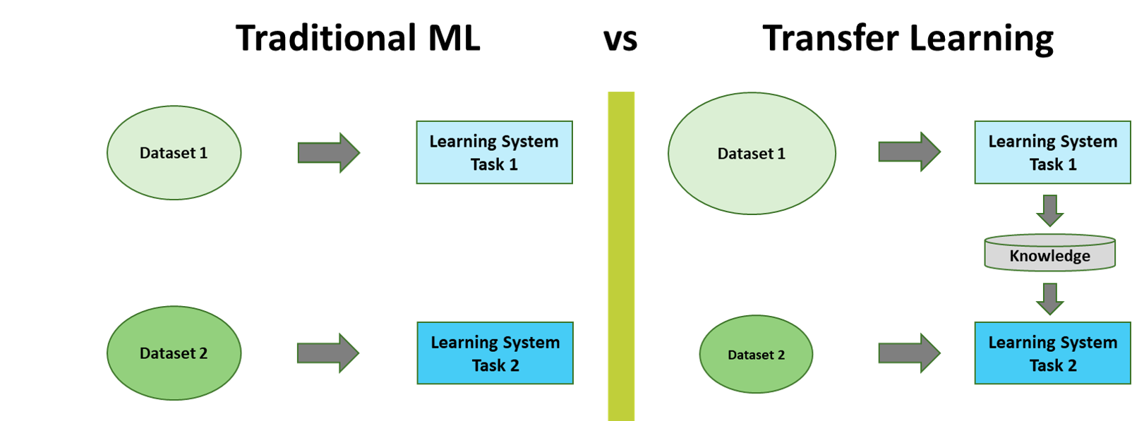
Figure 1: Traditional ML vs. Transfer Learning. Adapted from [14].
Transfer learning aims to mimic the human ability to acquire knowledge while learning one task and to then utilize this knowledge to solve some related task. The conceptual difference to traditional machine learning is displayed in Figure 1. In the traditional approach, for example, two models are trained separately without either retaining or transferring knowledge from one to the other. An example for transfer learning on the other hand would be to retain knowledge (e.g. weights or features) from training a model 1 and to then utilize this knowledge to train a model 2. In this case, model 1 would be called the source task and model 2 the target task [14].
To qualify as INDUCTIVE transfer learning, the source task has to be different from the target task and labeled data has to available in the target domain [13]. Both these definitional requirements are given in our specific case, with our source task being a language model (LM) and our target task (i.e. what we ultimately want to achieve) being a sentiment analysis. The Twitter dataset used for the latter is also labeled.
Quick note: A LM can predict the probability of the next word in a
sequence, based on the words already observed in this sequence (for a
more in-depth introduction to LMs, take a look at this
blog)
1.3. Our Datasets
For our source task (i.e. the LM) we chose the WikiText-103 dataset which consists of 28 595 preprocessed Wikipedia articles whose contents sum up to a total of 103 million words. For the sentiment analysis on the other hand, we selected the so-called Twitter US Airline Sentiment dataset. It contains 14 485 tweets concerning major US airlines. Based on the sentiment they convey, these tweets are labeled as either positive, negative or neutral. The dataset is imbalanced in that there are more negative than positive or neutral tweets (see Figure 2).
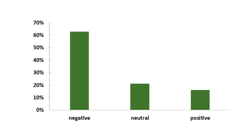
Figure 2: Sentiment Distribution in the
Twitter US Airline Sentiment Dataset.
With our project we aimed at not only giving an introduction to a state-of-the-art technique in text analysis but also at advancing the knowledge on and ultimately the practical application of ULMFiT. Bearing in mind that Howard and Ruder [10] have applied ULMFiT for sentiment analysis on Yelp and IMDb reviews with 25 000 to 650 000 examples, we consciously chose to use tweets for our project. We believe them to be not only considerably more colloquial but also substantially shorter (due to the limit of 140 characters per tweet) than the previously mentioned reviews. We hope that these differences will allow us to answer the following questions:
- Can ULMFiT really perform well on small datasets as Howard and Ruder claim?
- How well can knowledge be transferred from a source domain that is quite different to the target domain?
The original datasets can be found here:
1.4. Overview ULMFiT

Figure 3: Overview ULMFiT.
After having introduced the basic ideas underlying ULMFiT, we can now focus on the structure of the actual model. For the purpose of providing a general overview, the model can be split into three steps [10]:
- General-Domain LM Pretraining: In a first step, a LM is pretrained on a large general-domain corpus (in our case the WikiText-103 dataset). Now, the model is able to predict the next word in a sequence (with a certain degree of certainty). Figuratively speaking, at this stage the model learns the general features of the language, e.g. that the typical sentence structure of the English language is subject-verb-object.
- Target Task LM Fine-Tuning: Following the transfer learning approach, the knowledge gained in the first step should be utilized for the target task. However, the target task dataset (i.e. the Twitter US Airline Sentiment dataset) is likely from a different distribution than the source task dataset. To address this issue, the LM is consequently fine-tuned on the data of the target task. Just as after the first step, the model is at this point able to predict the next word in a sequence. Now however, it has also learned task-specific features of the language, such as the existence of handles in Twitter or the usage of slang.
- Target Task Classifier: Since ultimately, in our case, we do not want our model to predict the next word in a sequence but to provide a sentiment classification, in a third step the pretrained LM is expanded by two linear blocks so that the final output is a probability distribution over the sentiment labels (i.e. positive, negative and neutral).
In the following we are going to delve deeper into each of these three steps, beginning with the General-Domain LM Pretraining. As this section will already contain code snippets, it should be mentioned that the implementation is in great parts based on a library called fastai that sits on top of PyTorch. We mainly used open source code by Howard and Ruder [10], [15] and for the purpose of this blog post condensed portions of it into functions but also left out less relevant sections. If you are interested in the entire code, you can find it in our GitHub repository. To make sure the code runs smoothly, please take a look at the README file for instructions regarding the correct versions of the required libraries.
2. General-Domain Language Model Pretraining
As already described, in a first step a LM should be pretrained on the WikiText-103 dataset. Luckily Howard and Ruder [10] did exactly that and made the trained model available online, saving us a great amount of training time. For their LM they implemented a so-called AWD-LSTM - a regular LSTM to which several regularization and optimization techniques were applied. We are only going to introduce a couple of these techniques which are visible in our code snippets. If you would like to know more about AWD-LSTMs, we recommend Merity, Keskar and Socher’s [19] article where the method was originally introduced. While you can theoretically train your LM any way you prefer, AWD-LSTMs have been shown to produce state-of-the-art results in Language Modeling and are beginning to be widely used by other researchers, e.g. [16], [17]. If you are not yet familiar with LSTMs or need to refresh your memory, have a look at this blog.
Regarding the architecture of their AWD-LSTM, Howard and Ruder [10] chose an embedding size of 400, 3 layers and 1150 hidden activations per layer.
2.1. Word Embedding
What does an embedding size of 400 refer to? To answer this question it is crucial to understand word embeddings. Neural networks (or any machine learning algorithm for that matter) require language to be transformed to some sort of numerical representation in order to be processable.
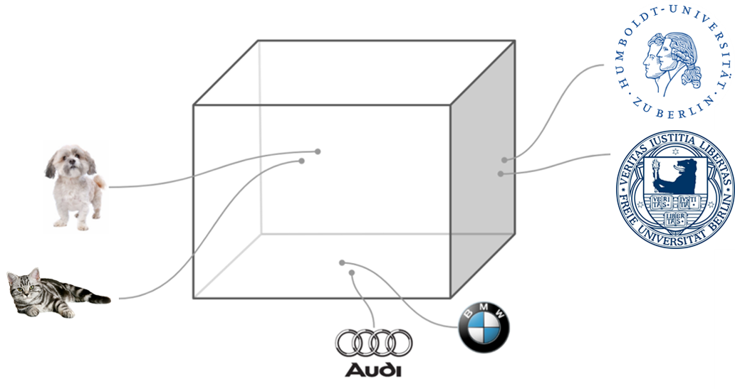
Figure 4: Word Embeddings. Adapted from [15].
Word embeddings enable the representation of words in the form of real-valued vectors in a predefined vector space [18]. If, for example, three dimensional vectors (i.e. the embedding size equals 3) are chosen to represent certain words, a possible vector space could look like the one in Figure 4. Such a dense representation is clearly superior to the high dimensionality of sparse word representations (e.g. one-hot encoding).
It is also important to note that these vectors capture the semantic relationship among words. Consequently, words, as for example "HU" and "FU" (abbreviations for Humboldt-Universität and Freie Universität), are closer to one another than "HU" and "cat". By using word embeddings we are also able to identify relations, such as: HU - Mitte + Dahlem = FU
In the case of our AWD-LSTM, the vectors representing the respective words are initialized in a so-called embedding layer and get updated while training the neural network. As already mentioned, the embedding size equals 400 in our case, i.e. we represent each word in our corpus in a 400-dimensional vector space.
2.2. Example of a Forward Pass through the LM
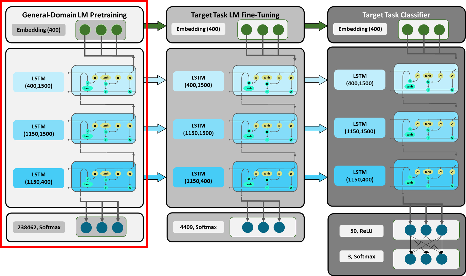
Figure 5: Detailed Overview ULMFiT: General-Domain LM Pretraining.
Adapted from [10].
Figure 5 displays a detailed overview of our ULMFiT model and provides an insight into each layer (the numbers in brackets refer to the dimensions of the inputs and outputs of the respective layer). While we will get to the second and third part of the model later, we will now show you an exemplary forward pass through the LM that was trained on the WikiText-103 dataset (i.e. the red-rimmed section). By taking a look at the respective inputs, mathematical computations and outputs, we hope to provide a better understanding of what exactly happens in each layer. We are going to use self-defined classes and functions from the code file ‘functions’, which we rebuilt to illustrate what happens inside the fastai library
For this purpose we start off by defining an exemplary sentence we are going to feed into the model.
Whether it be to train or test a LM, texts that are going to be passed through the model first have to be tokenized and encoded with an integer. The tokenize function automatically segments the running text into its tokens and adds a new line tag as well as a tag xbos to indicate the beginning of the text. The latter is particularly important when several distinct texts are fed into the model as they will all be concatenated. Since Howard and Ruder have already trained the LM on the WikiText-103 dataset, they also provide a ready-made list of all unique tokens in the dataset, ordered from most often to least often used (variable itos_wiki: “integer to string”) as well as the same information formatted as a dictionary (variable stoi_wiki: “string to integer”). Consequently loading this vocabulary and dictionary enables us to encode our exemplary sentence accordingly.
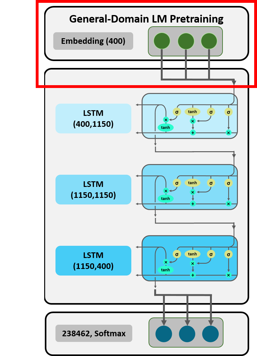
Figure 6: Embedding Layer.
At this point in time, the sentence enters the first layer of the LM, i.e. the embedding layer. The embedding matrix lm_wgts_wiki[‘0.encoder.weight’] (again, ready-made provided by Howard and Ruder) in our model has a dimension of 238 462 $\times$ 400 (embedding size equals 400 and number of unique tokens equals 238 462), i.e. one 400-dimensional vector for each token in the WikiText-103 dataset. The process of matching every encoded token of our exemplary sentence to its embedding vector is executed via one-hot encoding. Via the oneHot function we, thus, obtain a tensor of 13 vectors (with 13 being the number of tokens in our sentence) of size 1 $\times$ 238 462, each indicating which token of the vocabulary it represents. As the first of these vectors refers to the first token in the sentence, the second to the second and so on, this procedure also makes sure that the model understands the word order in the sentence.
In order to obtain the embeddings for each encoded token in the sentence, the one-hot encoded tensor is now multiplied with the embedding matrix, resulting in tensor of 13 vectors of size 1 $\times$ 400.
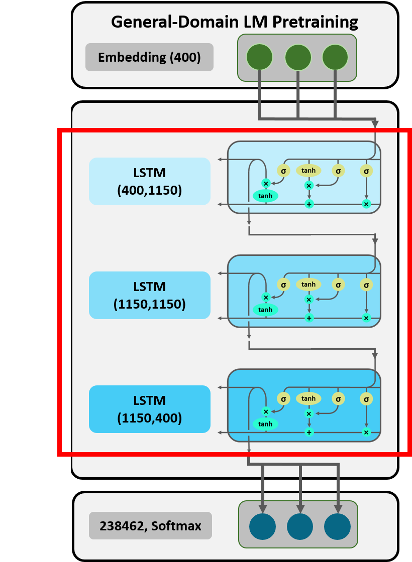
Figure 7: LSTM Layers.
After the embedding layer, the sentence is now passed through the three stacked LSTM layers. We defined the class LSTM to reveal their modus operandi. Since the focus of this demonstration lies on describing the memory and the hidden state, we exclude dropouts and further regularization techniques.
The mentioned class contains a function which performs the calculations within one LSTM and returns the output. To be precise, this function returns the hidden state after each token has been processd and arranges them in tensors (according to word order). Within the resulting tensors of shape 13 $\times$ 1 $\times$ 1150 (with 1150 being the number of hidden activations) each vector illustrates the respective hidden state after the model processed that token. For the hidden state vector of the first token there is no context information gathered yet. However, the later a word occurs in the sentence, the more memory of prior context is stored in the cell state and included in the hidden state.
The function stacked combines three individual LSTMs to obtain the model structure illustrated in Figure 7. Our tensor with the word embeddings is the input to the first layer (dimension: 13 $\times$ 1 $\times$ 400), whereas the following ones take the hidden states of the previous layer as input (dimension: 13 $\times$ 1 $\times$ 1150). Besides the model parameters, the created object st_lstm now stores hidden states for every layer.
The hidden state of the last layer has the same shape as the embedded input, i.e. a tensor of size 13 $\times$1 $\times$ 400.
Inverse to the embedding process, the output hidden state tensor of the LSTMs is now multiplied with a decoder matrix, shaped 400 $\times$ 238 462. Our decoded tensor has the same shape as our one-hot encoded tensor.

Figure 8: Softmax.
In a last step, the softmax function transforms all values in the decoded tensor into probabilities. For every token in the exemplary sentence, the 1 $\times$ 238 462 vector indicates the probability for every token in the WikiText-103 vocabulary to be the next token. For example the second vector contains the probabilities for which token could be the third token in the sentence based on the first two tokens.
The output below displays the ten most likely tokens to follow
“Yesterday I flew with a new airline and it was really”
2.3. Preparations for Fine-Tuning
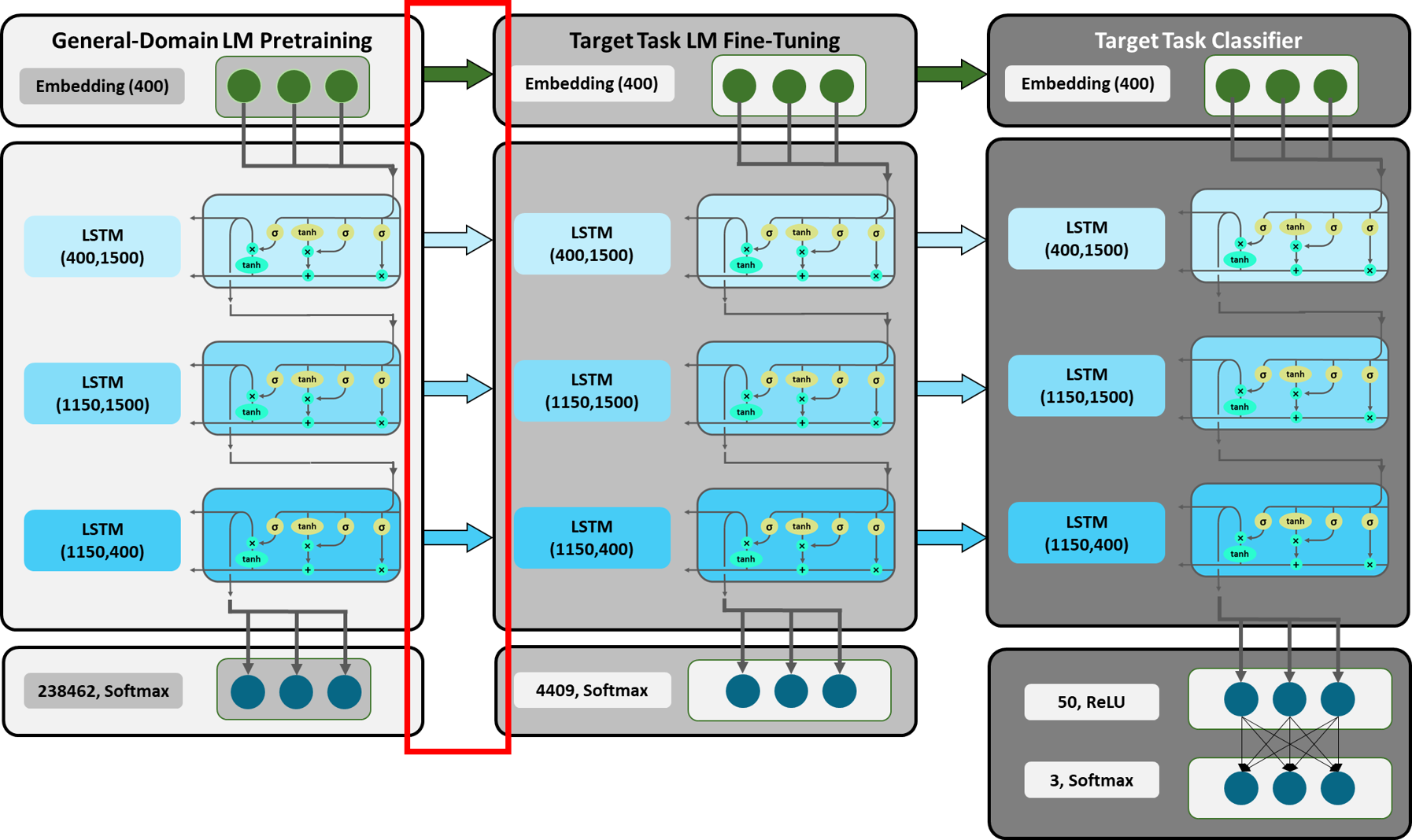
Figure 9: Detailed Overview ULMFiT: Preparations for Target Task LM
Fine-Tuning.
After having discussed the General-Domain LM Pretraining, we are now going to elaborate on the necessary steps to prepare for the Target Task LM Fine-Tuning. The latter is going to involve "retraining" the LM on the Twitter dataset. In preparation for this, the Twitter dataset has to be prepped and the model architecture of Howard and Ruder's AWD-LSTM has to be rebuilt in order to be able to load in the weights of the trained model the authors provided online.
The prepping of the Twitter US Airline Sentiment dataset involves data cleaning (e.g. the removal of links), the splitting into train and test datasets as well as the tokenization and encoding of all tweets. These steps will not be displayed here. As already described in section 2.2. of this blog post, we also require a vocabulary (itos) and dictionary (stoi) of the Twitter dataset. We could theoretically also combine the vocabulary of the WikiText-103 and our Twitter dataset instead of just using the latter for fine-tuning. However, the WikiText-103 vocabulary is huge (about 240 000 unique tokens) and a vocabulary size of more than 60 000 has been proven to be problematic for several implementations of ULMFiT [15]. If we chose to limit the combined vocabulary to the 60 000 most used tokens on the other hand, we would loose a substantial amount of Twitter specific tokens since these appear far less often owing to the Twitter dataset being fairly small. Consequently, we are only including the Twitter vocabulary (4409 unique tokens) and dictionary for the Target Task LM Fine-Tuning.
2.3.1. Matching Process for the Embedding Matrix
Before we recreate the architecture of the AWD-LSTM (embedding size of 400; 3 layers; 1150 hidden activations) and subsequently fill in the weights (lm_wgts_wiki) of the model trained on the WikiText-103 dataset, we have to adjust the embedding and the decoding matrix [10]. As previously shown, the embedding matrix enc_wgts trained on the WikiText-103 dataset is of size 238 462 $\times$ 400. Since we have chosen to only use the Twitter vocabulary for fine-tuning, the embedding matrix has to be adapted as it currently contains the embeddings for the 238 462 WikiText-103 tokens. For a better understanding of the changing dimensions and the necessity of the changes, please refer to section 2.2.
As displayed in Figure 10, all embeddings of tokens that do not occur in the Twitter dataset are deleted, while those that are part of both datasets remain unchanged. Tokens that can only be found in the Twitter dataset but not the WikiText-103 dataset obviously have not yet been embedded. Thus, they are assigned the row mean of all WikiText-103 embeddings.
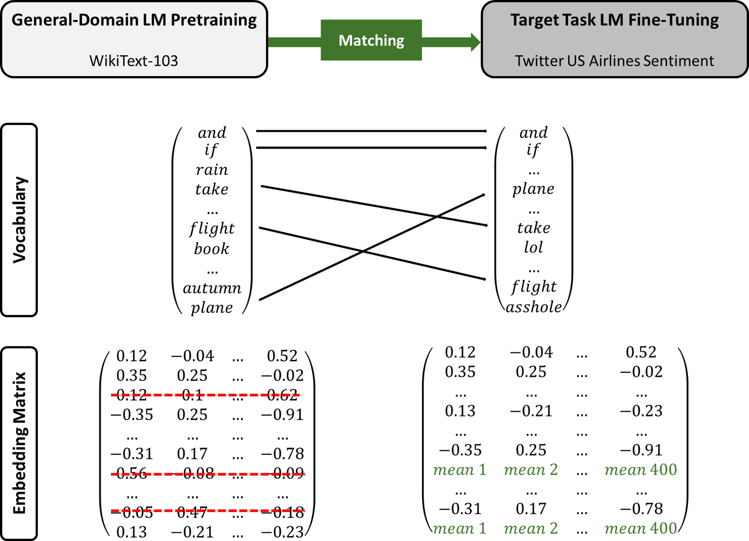
Figure 10: Matching Process for the Embedding Matrix.
Ultimately, the resulting embedding matrix is of size 4409 $\times$400 and overwrites the former embedding matrix. We also have to overwrite the decoding weights with the new embeddings as otherwise the mathematical operations shown in section 2.2. would not be possible (i.e. the dimensions have to match).
2.3.2. Variable Length Backpropagation Sequences
At this point we can begin to rebuild the architecture of the LM that was trained on the WikiText-103 dataset. In a first step we create data loaders for the training and validation data sets. These data loaders can be described as iterators that loop through mini-batches. For that purpose, we choose a batch size and backpropagation through time parameter. Backpropagation through time is the training algorithm used to update weights in a RNN. If you are not familiar with this, we recommend to read an introduction into the technique on this blog.
The concept behind mini-batches is displayed in Figure 11. As already
mentioned earlier, all tweets (whether in the training or validation
data set) will be concatenated before they are passed into the AWD-LSTM.
The immense size of this object makes the backpropagation through all of
it impossible in terms of memory capacities. Instead, the object is
split into a number of batches based on a certain batch size (bs). In
our case, the concatenated object would be split into 64 pieces. For
demonstration purposes you can imagine these batches being placed
underneath each other, resulting in a bs $\times$ number of tokens
in a batch sized matrix. As shown in Figure 11, mini-batches are then
created by truncating these batches according to the parameter bptt
which indicates how many tokens are going to be backpropagated through
when training the model. Thus, in our case one mini-batch comprises of
64 sequences of length 70. During the training process one mini-batch at
a time is going to be fed in the LM, i.e. 64 sequences are going to be
processed in parallel. This means that for each of these 64 sequences
the next tokens will be predicted and the loss calculated before the
backpropagation will begin. Following this, the next mini-batch will be
processed and so on. Exactly this iterative process is performed by a
data loader.
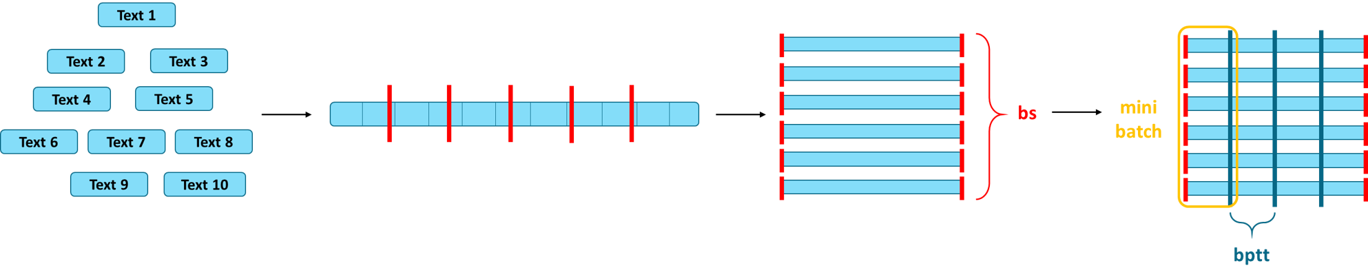
Figure 11: Mini-Batches. Adapted from [15].
Merity et al. [19] extended this technique by introducing **variable length backpropagation through time**. The main problem with the previously described method for creating mini-batches is that epoch for epoch exactly the same sequences of words are being backpropagated through. Variable length backpropagation through time tackles this issue by introducing a certain degree of randomness. When truncating the batches to mini-batches, 95% of the time *bptt* will be set to its original value (in our case 70) but 5% of the time a random number is chosen from a normal distribution. Consequently, different combinations of tokens will be backpropagated through. Ultimately, this facilitates a more efficient use of the existing data. This technique is included in fastai's data loader.
The next important step to recreate the architecture of the AWD-LSTM is to initialize the class LanguageModelData. We provide it with important information: The path where it should save all temporary and final models, how the padding token is encoded (1 in our case), the training and validation dataloaders we just created, as well as the batch size and backpropagation through time parameter. Padding is very relevant in our case since the model expects to be fed sequences of the same length which might not always be the case due to the process of creating mini-batches and using variable length backpropagation through time. Shorter sequences are thus padded with the encoded token 1 to reach the same overall length.
2.3.3. Adam Optimizer
As the optimization algorithm we choose the so-called Adam. Howard and Ruder [10] found this algorithm to work particularly well for NLP tasks when the parameters are set in an appropriate way. Adam can be described as an extension of Stochastic Gradient Descent and as an adaptive learning rate method. It estimates the first and second moments of the gradient to adapt the learning rate for each weight of a neural network. These moments are estimated by moving averages of the gradient and squared gradient (numerator) which are corrected for a certain bias (denominator) [20]:
$\begin{equation*} m_t = \frac{\beta_1 m_{t-1}+(1-\beta_1)g_t}{1-\beta_1^t} \\ v_t = \frac{\beta_2 v_{t-1}+(1-\beta_2)g_t^2}{1-\beta_2^t} \\ \end{equation*}$
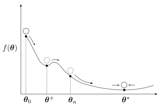
Figure 12: Adam Optimizer. Reprinted from [27].
(m, v: moving averages; g: gradient on current mini-batch; betas: hyper-parameters)
The concept behind Gradient Descent is often illustrated by means of a ball rolling down a slope (e.g. here) which should ultimately end up in the lowest valley (i.e. the global minimum). Using the same analogy, one could describe Adam as a heavy ball with friction [27]. As shown in Figure 12, it thus overshoots local minima and tends to settle at flat minima due to its mass.
As already mentioned, Howard and Ruder [10] suggest a specific setting for the parameters $\beta_1$ and $\beta_2$. Particularly, the default of 0.9 for $\beta_1$ should be reset to a value between 0.7 and 0.8.
2.3.4. Dropout
One regularization technique that is an essential part of AWD-LSTMs and applied in numerous forms throughout the model is called dropout. During the training of a neural network and thus the updating of weights to reduce the loss, some units may change in a way that they fix up the mistakes of the other units. This leads to complex codependencies, called co-adaptations and these co-adaptations do not generalize well to new data and, thus, provoke overfitting. One approach to reduce overfitting could be to fit all possible different neural networks on the same dataset and to average the predictions from each model. Since this is obviously not feasible in practice, the idea is implemented with dropout [21].
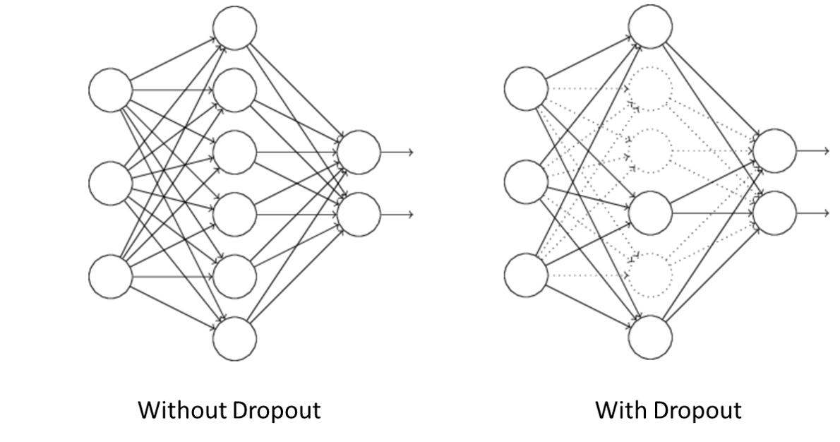
Figure 13: No Dropout vs. Dropout. Adapted from [22].
Dropout means that some of the units in a neural network are randomly deleted, as displayed in Figure 13. Following this, for one mini-batch the forward and backward pass are performed and the weights are updated. The deleted units are then restored and others are randomly chosen to be deleted next. This procedure is repeated until the training is completed. Of course, the final weights have been learned under different conditions than when new data is processed (because then the network can access all units). Therefore, the weights have to be adjusted, depending on the dropout rate. E.g. if the dropout rate equals 0.5 the weights have to be rescaled by half in the end. Since one unit cannot rely on the presence of particular other units, there are less co-adaptations [22].
For our LM we apply five different dropout methods, e.g. by setting certain rows of the embedding matrix to zero so that the model learns not to depend on single words. For details on the other forms of dropout in the AWD-LSTM, please refer to Merity et al. [19]. Fortunately, we do not have to search for the perfect combination of all of these parameters, since Howard [15] found that the following proportion of dropouts performs well. Thus, we merely have to choose a scaling parameter between 0 and 1 which is set to 0.7 in our case. In case of overfitting, we could for example increase this parameter.
Finally, we can build our model architecture. We do so by calling the method get_model of the LanguageModelData class. With this method we can apply all the attributes and functions we need to train our model, predict and so on. We provide our chosen optimizer, embedding size, number of hidden layers, number of hidden activations and dropout. Based on this information, our AWD-LSTM is built layer by layer by grabbing a PyTorch neural network model.
3. Target Task Language Model Fine-Tuning
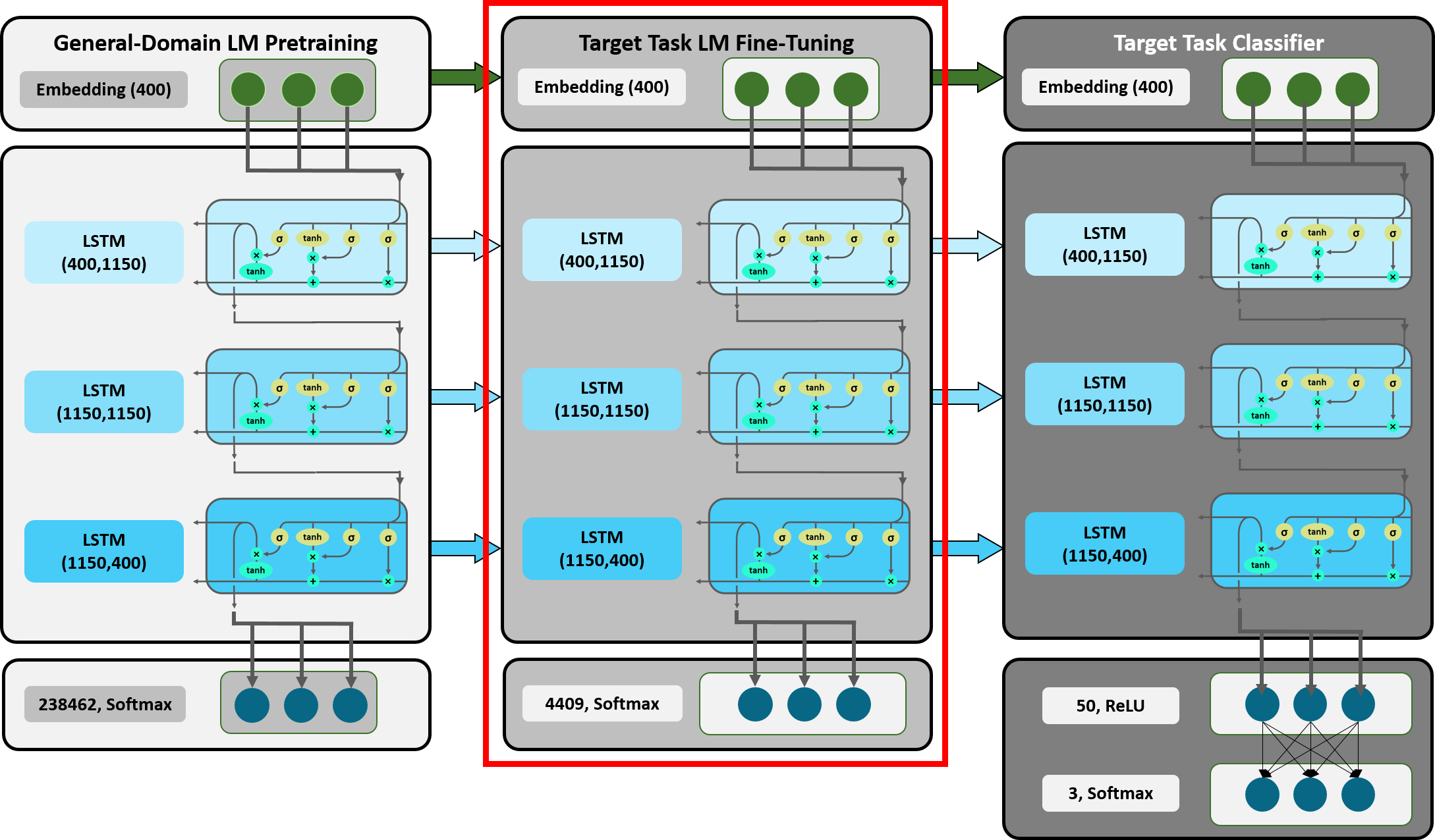
Figure 14: Detailed Overview ULMFiT: Target Task LM Fine-Tuning.
After we have made all the necessary provisions, we can now begin with the actual LM fine-tuning. It should be mentioned that while Howard and Ruder [10] were not the first to apply inductive transfer via fine-tuning in NLP, they were one of the first to do so successfully with regard to performance and efficiency. In previous attempts, the process of fine-tuning led to overfitting when datasets were small and even catastrophic forgetting with regard to the knowledge gained from the source task. Howard and Ruder solved these issues by introducing novel NLP-specific fine-tuning methods. Since these methods are an essential part of what makes ULMFiT a state-of-the-art technique, we are also going to expand on them as well.
3.1. Freezing
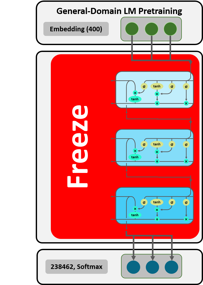
Figure 15: Freezing.
Since we transformed the embedding matrix in major ways (see section 2.3.1), part of our embedding (and decoding) layer is untrained with initial random weights (i.e. the row means of the WikiText-103 embedding matrix). If we now trained the entire model, we would risk catastrophic forgetting in our three LSTMs. Therefore, in a first step, we “freeze” the weights of the LSTM layers and train the rest of the model for one epoch. Thus, only the embedding and decoding weights are trained, in order to adjust them to the LSTM weights. This technique, called freezing, was introduced by Felbo et al. [23] and is implemented by the function freeze_to(-1). For the second step all layers are unfrozen so that also the LSTM layers can be fine-tuned.
We will illustrate the concept of freezing by showing the model weight matrices after each step. The first output displays the weights pretrained on the WikiText-103 dataset whose embedding and decoding weights have been adjusted in section 2.3.1..
3.2. Learning Rate Schedule

Figure 16: Slanted Triangular LRs.
For our model we apply a learning rate (LR) schedule which means that the LR does not remain constant across the iterations in the training process but is adjusted. We start of with a short steep increase in size of LRs to quickly converge to a suitable region in the parameter space and a long decay period to precisely fine-tune the weights. This particular approach of adjusting the LR is called slanted triangular LRs [10] and is inspired by cyclical LRs which Smith [24] has introduced.
Slanted triangular LRs are implemented in the fit function by use_clr. The first parameter represents the ratio of highest to lowest LR, the second the ratio of decaying to increasing periods. We merely have to set the value for the starting LR, which we do here with 0.001.
As described before, we are now training our frozen model for one epoch.
When checking the updated weights in our model, the freezing becomes obvious, as only encoder and decoder weights changed while those of the LSTM layers remained the same.
In a next step all layers are unfrozen in order to train the entire model. Before this phase can begin, it is necessary to find an adequate peak LR. A procedure, also introduced by Smith [24], has been proven to be very useful for this purpose.
Followings his approach, we conduct an “exploratory training process”. We start off with our initial weights and update them with a very small initial LR, in our case. In our case we do so for all LRs in between 0.000001 and 1. With learner.sched.plot() the LRs can be plotted against the loss. Using this plot, we can check how big the LR can grow so that the descent of the loss is still big enough. Based on our own visual judgement, we set the peak LR to the highest LR in the area where the loss has its sharpest descent. In our case this seems to be 0.01.
3.3. Discriminative Fine-Tuning
As already described, our AWD-LSTM contains three stacked LSTMs. Yosinski et al. [25] found, that such a stacked structure is particularly valuable when working with data as complex as text since it is capable of capturing different types of information at every level, starting with general information on the first one and growing more and more specific on every further layer. In the textual data context, the first layer might catch information like basic sentence structure, while the next ones dig deeper, such as the workings of different tenses.
These differences in processing can be addressed by using different LRs depending on the respective layer. Usually, the model parameters $\theta$ are updated during the training process with a fixed LR $\eta$ [26]:
$ \begin{equation*} \theta_{t} = \theta_{t-1} - \eta \nabla_{\theta} J(\theta) \end{equation*} $
In the discriminative approach, each layer has its own LR $\eta^{l}$:
$ \begin{equation*} \theta_{t}^{l} = \theta_{t-1}^{l} - \eta^{l} \nabla_{\theta^{l}} J(\theta) \end{equation*} $
Starting with a small LR in the first LSTM, it increases through the layers due to the increasing amount of acquired knowledge and information complexity. In the code we define a numpy array with the exponentially increasing LRs, starting with the smallest one for the first LSTM.
After training the model for three epochs, the accuracy on the validation dataset is about 30 percent. While this may seem low at first glance, one has to keep in mind that the predicted word is part of a vocabulary of 4409 possible next tokens. However, we do not quite reach Howard’s [15] 31 percent when training the LM on the well known IMDb dataset. This might be owed to the much smaller dataset we use compared to his.
Reviewing the model weights one last time, we can see that in this step all parameters were trained.
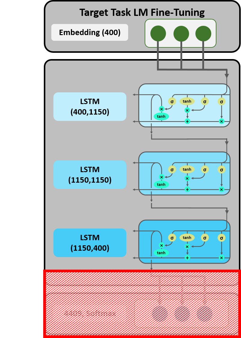
Figure 17: Cut-Off.
Our LM has now learned task-specific features of the language. However,
in order for this model to be capable of sentiment analysis, its
architecture needs to be adjusted. At the same time, the knowledge
gained from training the LM has to be preserved. As displayed in Figure
17, the embedding layer and the three LSTMs are, therefore, adopted from
the LM, while the decoder and the softmax layer are cut off. This step
is executed by the save_encoder command.
4. Target Task Classifier
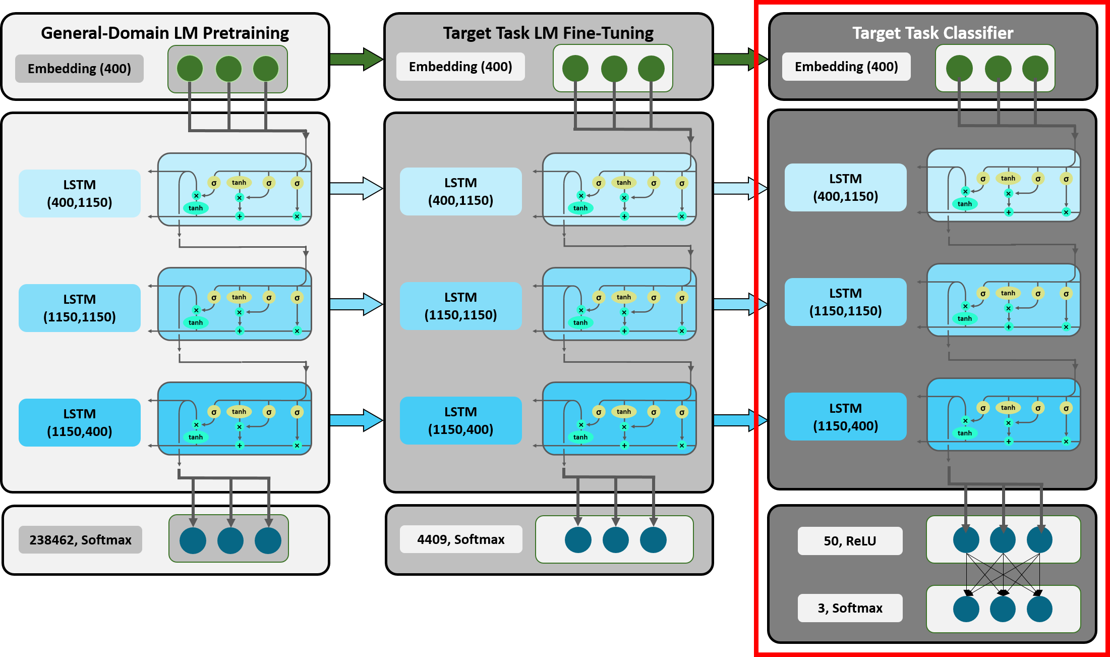
Figure 18: Detailed Overview ULMFiT: Target Task Classifier.
In the final stage of ULMFiT, we are now going to perform our actual target task, the sentiment classification. As already mentioned, the LMs architecture has to be adjusted to do so. Two linear blocks with a ReLU activation function and a softmax activation respectively are added on top of the LSTM layer (see Figure 18). The softmax layer ultimately outputs probabilities for each label (positive, negative or neutral) of the corresponding tweet. Applied methods, the architecture of the classifier and input as well as output dimensions will be discussed in the following.
When feeding mini-batches into the LM (see section 2.3.2.), some of the sequences might contain one tweet and half of another tweet. Such an input could not be fed into the classifier as it needs to predict the label for each tweet separately. Consequently, each mini-batch contains sequences consisting of one entire tweet. Thus, each tweet passed through the embedding layer and LSTM is represented by a tensor containing embedding vectors for each token. If we consider an example tweet, then similar to the LM the output tensor of the last LSTM has a number of vectors equal to the number of tokens in the document and again each embedding vector is of dimension 400. This output tensor is the last hidden state of the tweet, meaning that every token of the tweet has been fully processed in the LSTM layer.
In the first step of code implementation, the model data is defined. The function data_loader, based on fastai sampling techniques, performs several tasks at a time. A data loader takes the encoded tweets and their corresponding labels, returns them as a tuple and sorts them in a way that the shortest documents are placed on top. Sorting documents by length mainly reduces the amount of padding and ultimately saves computation time. Technically, encoded tweets are padded with the index 1 to the same length as the longest document in the mini-batch. As elaborated on before, the data loader takes care of iterating the mini-batches through the model.
4.1. Concat Pooling
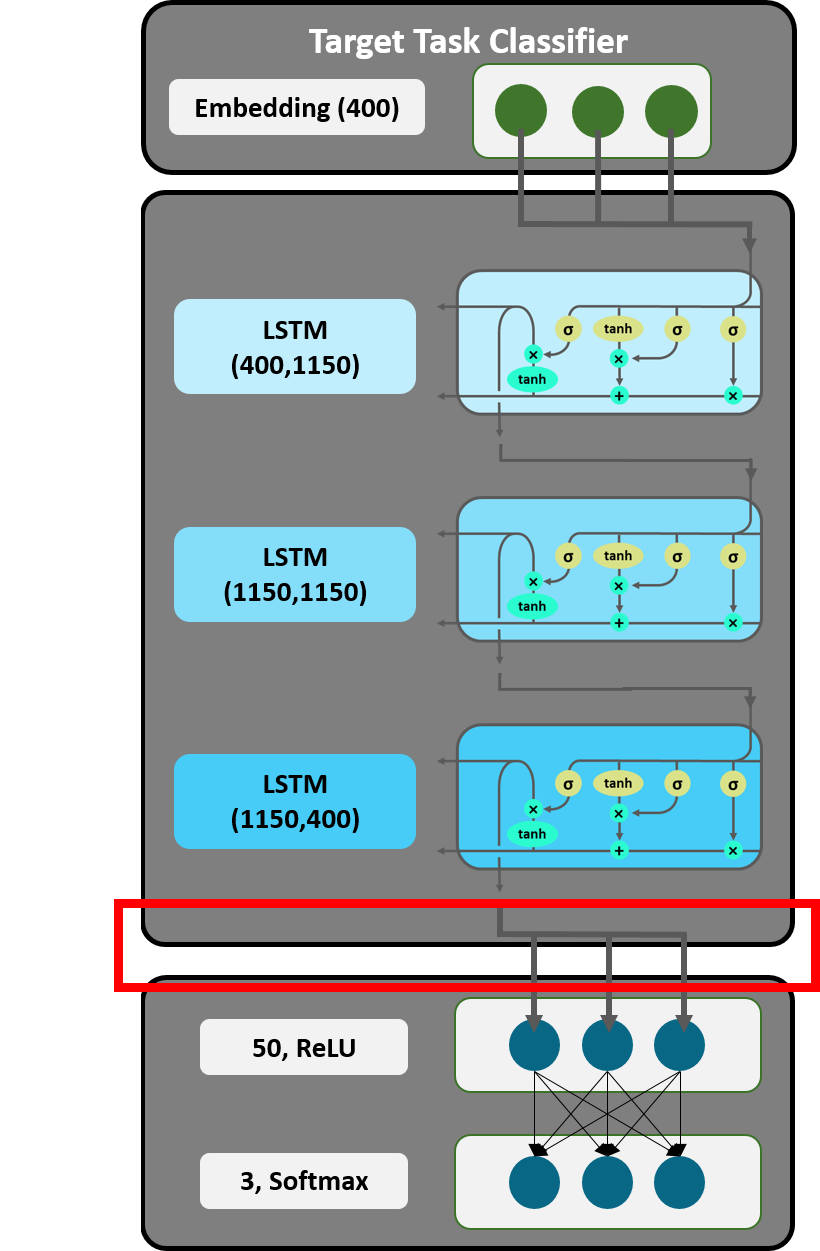
Figure 19: Concat Pooling.
Usually some of the words in an input document contain more relevant information for the classification than others. After each time step (in this case processing one word in a LSTM layer) the hidden state of the document is updated. During this process information may get lost, if only the last hidden state is considered. Concat Pooling, a technique introduced by Howard and Ruder [10], tackles the problem of catastrophic forgetting and takes information throughout time steps into account. In other words, the last hidden state is concatenated with a max-pooled and a mean-pooled representation of the hidden states.
The max-pooled representation is generated by collecting the largest values for each of the 400 features over all hidden states of a document (in our case a tweet) in the third LSTM layer, whereas mean-pool calculates the average of each of the 400 features. As displayed in Figure 20 (hidden state: h; time steps: 1 … T) both approaches return vectors of dimension 1 $\times$400 and concatenation results in 1 $\times$1200 feature vectors for each word. Following this, they can be passed as a tensor to the decoder.
4.2. Linear Decoder
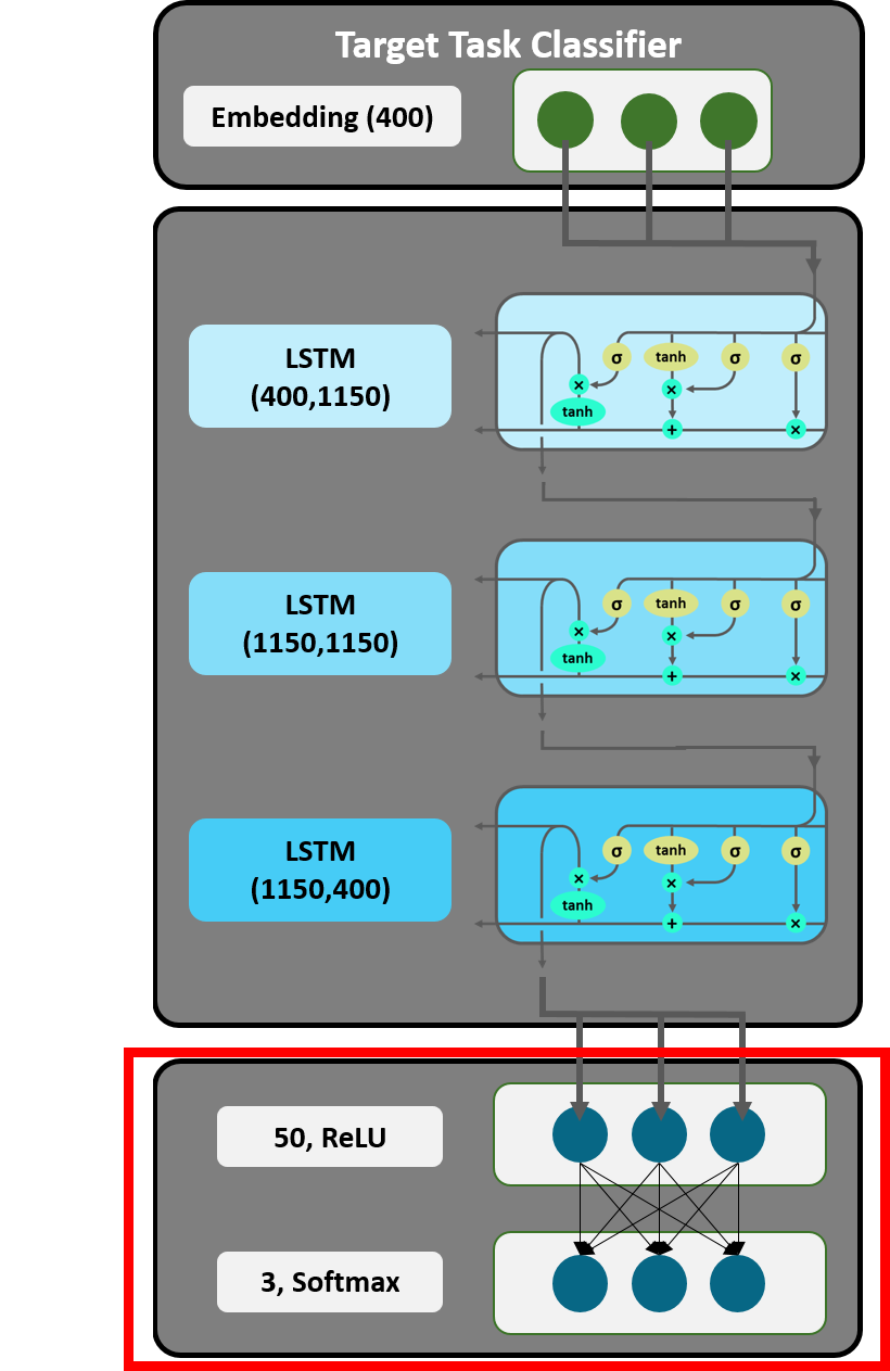
Figure 20: Linear Decoder.
The linear decoder works as a feedforward neural network, which applies a ReLU and Softmax activation function on the concat-pooled tensor. In the ReLU layer with 50 activations, each vector of the tensor is multiplied by a randomly initialized weight matrix and subsequently reduced to the dimension of 50. The softmax layer further reduces the dimension to 3 and returns probabilities by scaling output values between 0 and 1. In a last step, a cross entropy loss function determines the loss and an Adam optimizer is applied. Weights are adjusted accordingly.
Regarding the implementation, we can now build the architecture of the Target Task Classifier with the function get_rnn_classifier(). Embedding layer and LSTM layers are rebuilt by using the fastai MultiBatchRNN Encoder, which also adds dropouts to the layers. In order to build an equivalent embedding matrix and LSTM to our LM, the hyperparameters remain the same. After having recreated the LM’s architecture the weights from our previously trained model can be loaded in and thus, weights do not have to be randomly initialized.
In order to build the linear decoder on top of the LSTM, the PyTorch container SequentialRNN is used to add modules in the order they are passed to it. PoolingLinearClassifier is a class that contains the previously discussed Concat Pooling, done by PyTorch functions (adaptive_max_pool1d; adaptive_avg_pool1d). Furthermore, it adds the two linear blocks with dropouts and Batch Normalization to the model. A ReLU activation function is assigned to the first linear block. However, the softmax activation of the output layer is combined with the cross entropy loss function, defined by another PyTorch module in the RNN_Learner class.
The resulting object is now passed to a learner that actually trains the classifier. Whereas LRs defines the step size (towards a minimum), learn.clip limits the size of the actual update of the weights in the model. Thus, it prevents overly aggressive updating.
4.3. Gradual Unfreezing
As mentioned before, two linear blocks are added on top of the embedding layer and the LSTM. Since the linear layers are initialized by randomly distributed weights and therefore risk catastrophic forgetting in training, it makes sense to use the freezing method again. In doing so, the new linear layers are fine-tuned before the entire model gets fine-tuned. As displayed in Figure 21, in the first epoch of training, all layers but the softmax output layer are frozen and weights of frozen layers will not be updated. During the next epoch, the ReLU layer is unfrozen and fine-tuned as well. In all following epochs the entire model is fine-tuned.
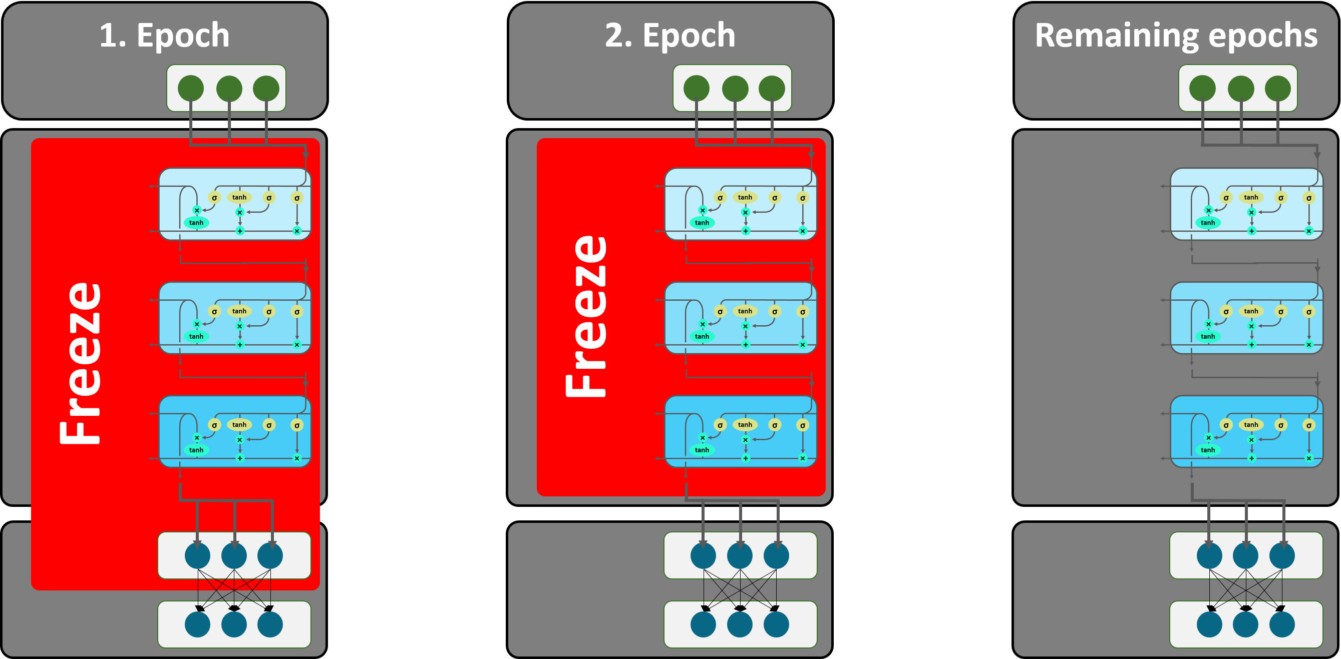
Figure 21: Gradual Unfreezing.
After the lr_find algorithm we set our learning rate schedule and get an accuracy of 84%.
4.4. Benchmarks
After training the entire model for six epochs, the classifier achieves an accuracy of around 83%. How good is this result compared to possible benchmarks?
For this purpose, we can consider a probabilistic as well as a random approach. Since our dataset is imbalanced with around 60% of the tweets labeled negative, assigning a tweet to this label is most likely. This method would result in an accuracy of 60%. If we just randomly drew labels for each tweet, every third tweet would be guessed right on average. Hence, the classifier model clearly outperforms both these benchmarks.
Comparing our results to other approaches on the same datasets Kaggle, the ULMFiT model is clearly superior in terms of accuracy:
- Support Vector Machine (SVM) - 78.5%
- Bag-of-words SVM - 78.5%
- Deep Learning Model with Dropouts in Keras - 77.9%
- Our result - 84.1%
In the beginning of this blog post we asked the following questions:
- Can ULMFiT really perform well on small datasets as Howard and Ruder claim?
- How well can knowledge be transferred from a source domain that is quite different to the target domain?
The results of our project indicate that ULMFiT indeed provides state-of-the-art results even with a dataset as small as our Twitter US Airline Sentiment. In addition to that the disparity between source and target domain does not appear to impair performance.
4.5. Example of a Forward Pass through the Classifier
As for the LM, we implemented an exemplary forward pass through the classifier. Firstly, the vocabulary of the fine-tuned Twitter US Airline Sentiment dataset and the model weights of the classifier we just trained are loaded. Following this, the prep function from the Classifier class executes tokenization, one-hot encoding, embedding and LSTM forward pass, which was already explained earlier for the Wikitext-103 model. The output of this function is the hidden state tensor of the last LSTM layer with the shape of 13 $\times$ 1 $\times$ 400.
In the next step, we apply Concat Pooling for the last hidden state vector of the tensor, which represents the last word and contains the remembered information about all previous words. The resulting vector has a size of 400 multiplied by three.
In the next layer, the Concat Pooled output vector is scaled down to the length of 50 and processed by a ReLU function.
Eventually, the Classifier function clas_predict scales the vector down to our 3 classes and performs a softmax activation in order to obtain the probabilities for the three classes.
5. Our Model Extension
In the very beginning of our project, we contemplated pretraining our own LM, instead of using Howard and Ruder’s WikiText-103 LM. For that purpose, we intended to use the Sentiment140 dataset which consists of about 1.6 million English tweets that cover a wide range of topics (and can be found here). We believed that due to the similarity of the source and target domain, we might achieve a better overall performance. However, we quickly reached the limit of memory capacities available to us. At this point we cycled back to the idea of transfer learning. As already elaborated on, one of the problems transfer learning tackles is the time and resource consuming nature of training models from scratch.
Consequently, we decided to use Howard and Ruder’s LM that was trained on WikiText-103 for the General-Domain LM Pretraining but to then fine-tune this model with 300 000 tweets from the Sentiment140 dataset (a process we call Target-Domain LM Fine-Tuning). This intermediate step was then followed by the usual fine-tuning with the Twitter US Airline Sentiment dataset as well as the transformation into a classifier. Figure 22 displays the structure of our model extension.
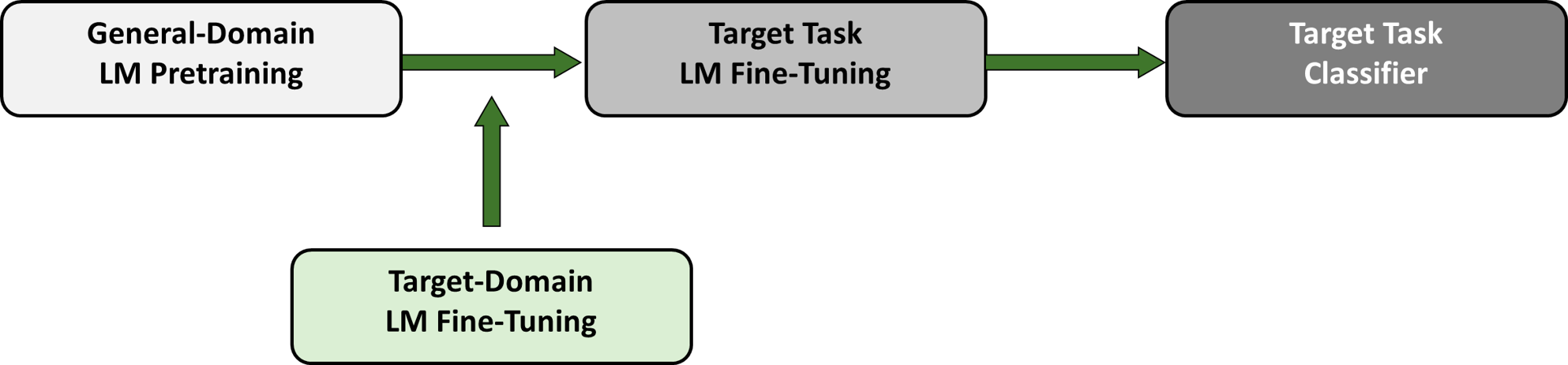
Figure 22: Our Extension of ULMFiT.
Researchers and practitioners alike are often faced with the problem of not having enough labeled data for text classification tasks. Since it does not require labeled data, we believed that Target-Domain LM Fine-Tuning might be a useful and easy to implement tool to boost performance by making up for a small target task dataset. Since we also had a fairly small target task dataset for our project that tended to overfit rather fast, we expected the huge Sentiment140 dataset to improve the LM, i.e. to improve its knowledge of Twitter slang by means of its many examples. The improved LM should then also allow for a better sentiment classification.
5.1. Results
In the following, we are going to examine the results of the experiments regarding our model extension. Table 1 displays the accuracy of the LM after the Target-Domain LM Fine-Tuning (i.e. the Target Task LM Fine-Tuning had not yet been performed). An accuracy of about 27% is a fairly good result. What is, however, far more interesting is to compare the results of the original ULMFiT and the extended version.
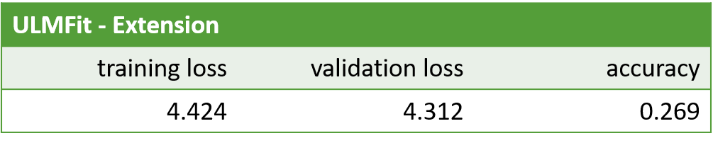
Table 1: Results LM Post Target-Domain LM Fine-Tuning.
As displayed in Figure 23 we are first going to compare the perfomance of the original vs. the extended ULMFiT at the step of Target Task LM Fine-Tuning when only the embedding layer had been trained.
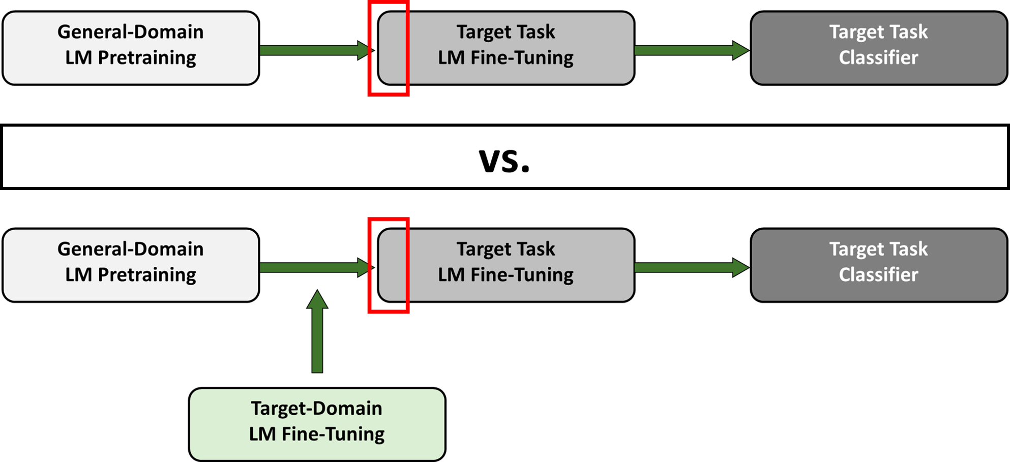
Figure 23: Our Extension of ULMFiT: Results Post Training the LM Embedding Layer
The considerably higher accuracy of the LM in the extended ULMFiT, shown in Table 2, seems to confirm our intuition that due to the fine-tuning with the Sentiment140 dataset the LM has already learned a significant amount of “Twitter slang” compared to the original ULMFiT at the same stage.

Table 2: Results Post Training the LM Embedding Layer.
However, after we trained the latter for a couple of epochs it quickly caught up to the extended version and ultimately both LMs achieved approximately the same accuracy. Both models also performed equally well with regard to the sentiment classification as displayed in Table 3. For the moment, we can, thus, not detect any significant improvements by extending the ULMFiT model.

Table 3: Results Post Training the LM Embedding Layer.
5.2. Without Vocabulary Reduction
As our first experiments did not show any benefits of adding an additional step to the ULMFiT model, we slightly changed our approach. As explained in section 2.3.1., when fine-tuning the LM of the original ULMFiT we only used the Twitter US Airline vocabulary. In our extended model we also only used the Sentiment140 vocabulary in the first fine-tuning step and only the Twitter US Airline vocabulary in the second fine-tuning step.
Now, however, we wanted to investigate whether it might be beneficial for the performance of the extended model to keep the Sentiment140 vocabulary in addition to the Twitter US Airline vocabulary for the Target Task LM Fine-Tuning. As the combined vocabulary has less than 60 000 unique tokens, there should be no losses in efficiency. Due to the increased vocabulary, we assumed that less tokens in the validation dataset might be assigned the token for unknown words and subsequently, the performance in the LM and ultimately the classifier might improve compared to the results for the extended model in Table 2 and 3. However, the results in Table 4 do not confirm our assumptions.

Table 4: Results Post Target Task LM Fine-Tuning.
Even though combining the vocabularies does not seem to make a difference for the accuracy regarding the sentiment classification of the airline tweets, it might make a difference, if we feed a new dataset into our trained model. Again, due to the increased vocabulary, completely unknown data might be better classified in our extended model than in the original ULMFiT. To test this hypothesis, we used the First GOP Debate Twitter Sentiment dataset which consists of almost 14 000 tweets about the first GOP debate in the 2016 presidential election in the US. The dataset can be found here. Since this dataset and our Twitter US Airline Sentiment dataset are thematically very different we expected mediocre results either way. As displayed in Table 5 this was indeed the case with results worse than our benchmark (60% of all tweets are negative) but in addition to this, we could, again, not detect any notable difference between the original and extended model.
Table 4: Results GOP Sentiment Classification.
6. Conclusion
We hope this blog post gave you a comprehensive overview of ULMFiT and what makes it such a state-of-the-art technique, from inductive transfer learning, to useful regularization and optimization techniques and to new NLP specific fine-tuning methods. If you are now just as enthusiastic about ULMFiT as we are, have a go at training your own ULMFiT on new datasets or try experimenting with your own model extensions! Whether in regard to novel applications or further techniques, there are numerous ways to go beyond what we did in this blog post, e.g by applying ULMFiT to non-English datasets or by implementing a bidirectional LM to boost performance [10].
Both the research on ULMFiT and the implementations in the fastai library are constantly evolving. Regarding the latter, Howard is for example currently working on implementing hyperparameter tuning. In terms of the former, researchers have started to investigate the applicability of ULMFiT for various scenarios [28],[29]. When looking at NLP on a larger scale, it seems likely that the field will continue to discover and customize approaches proven successful in CV (e.g. data augmentation).
7. Reference List
[1] Sebastian Ruder, NLP’s ImageNet moment has arrived, The Gradient, Jul. 8, 2018, https://thegradient.pub/nlp-imagenet/ [Blog]
[2] Tom Young, Devamanyu Hazarika, Soujanya Poria and Erik Cambria, Recent Trends in Deep Learning Based Natural Language Processing, IEEE Computational Intelligence Magazine, vol. 13, issue 3, pp. 55-75, Aug. 2018
[3] Tomas Mikolov, Ilya Sutskever, Kai Chen, Greg Corrado and Jeffrey Dean, Distributed Representations of Words and Phrases and their Compositionality, arXiv:1310.4546v1 [cs.CL], Oct. 16, 2013
[4] Jeffrey Pennington, Richard Socher and Christopher D. Manning, GloVe: Global Vectors for Word Representation, Computer Science Department, Stanford University, 2014
[5] Matthew E. Peters, Waleed Ammar, Chandra Bhagavatula and Russell Power, Semi-supervised sequence tagging with bidirectional language models, arXiv:1705.00108v1 [cs.CL], Apr. 29, 2017
[6] Arvind Neelakantan, Jeevan Shankar, Alexandre Passos and Andrew McCallum, Efficient Non-parametric Estimation of Multiple Embeddings per Word in Vector Space, arXiv:1504.06654v1 [cs.CL], Apr. 24, 2015
[7] Bryan McCann, James Bradbury, Caiming Xiong and Richard Socher, Learned in Translation: Contextualized Word Vectors, arXiv:1708.00107v2 [cs.CL], Jun. 20, 2018
[8] Kaiming He, Georgia Gkioxari, Piotr Dollár and Ross Girshick, Mask R-CNN, arXiv:1703.06870v3 [cs.CV], Jan. 24, 2018
[9] Joao Carreira, Andrew Zisserman, Quo Vadis, Action Recognition? A New Model and the Kinetics Dataset, arXiv:1705.07750v3 [cs.CV], Feb. 12, 2018
[10] Jeremy Howard, Sebastian Ruder, Universal Language Model Fine-tuning for Text Classification, arXiv:1801.06146, Jan. 18, 2018
[11] Matthew E. Peters, Mark Neumann, Mohit Iyyer, Matt Gardner, Christopher Clark, Kenton Lee and Luke Zettlemoyer, Deep contextualized word representations, arXiv:1802.05365v2 [cs.CL], Mar. 22, 2018
[12] Alec Radford, Karthik Narasimhan, Tim Salimans and Ilya Sutskever, Improving Language Understanding by Generative Pre-Training, OpenAI Blog, Jun. 11, 2018
[13] Sinno Jialin Pan, Qiang Yang, A Survey on Transfer Learning, IEEE Transactions on Knowledge and Data Engineering, vol. 22, issue 10, Oct. 2010
[14] Dipanjan Sarkar, A Comprehensive Hands-on Guide to Transfer Learning with Real-World Applications in Deep Learning, Towards Data Science, Nov. 14, 2018 [Blog]
[15] Jeremy Howard, Lesson 10: Deep Learning Part 2 2018 - NLP Classification and Translation, https://www.youtube.com/watch?v=h5Tz7gZT9Fo&t=4191s%5D, May 7, 2018 [Video]
[16] Ben Krause, Emmanuel Kahembwe, Iain Murray and Steve Renals, Dynamic Evaluation of Neural Sequence Models, arXiv:1709.07432, Sep. 21, 2017
[17] Zhilin Yang, Zihang Dai, Ruslan Salakhutdinov and William W. Cohen, Breaking the Softmax Bottleneck: A High-Rank RNN Language Model, arXiv:1711.03953, Nov. 10, 2017
[18] Jason Brownlee, What Are Word Embeddings for Text?, Machine Learning Mastery, posted on Oct. 11, 2017, https://machinelearningmastery.com/what-are-word-embeddings/
[19] Stephen Merity, Nitish Shirish Keskar, Richard Socher, Regularizing and Optimizing LSTM Language Models, arXiv:1708.02182v1 [cs.CL], Aug. 8, 2017
[20] Diederik P. Kingma, Jimmy Ba, Adam: A Method for Stochastic Optimization, arXiv:1412.6980v9 [cs.LG], Jan. 20, 2017
[21] Nitish Srivastava, Geoffrey Hinton, Alex Krizhevsky, Ilya Sutskever and Ruslan Salakhutdinov, Dropout: a simple way to prevent neural networks from overfitting, The Journal of Machine Learning Research, vol. 15, issue 1, pp. 1929-1958 Jan. 2014
[22] Michael Nielsen, Improving the way neural networks learn, Neural Networks and Deep Learning, posted in Oct. 2018, http://neuralnetworksanddeeplearning.com/chap3.html
[23] Bjarke Felbo, Alan Mislove, Anders Søgaard, Iyad Rahwan and Sune Lehmann, Using millions of emoji occurrences to learn any-domain representations for detecting sentiment, emotion and sarcasm, arXiv:1708.00524v2 [stat.ML], Oct. 7, 2017
[24] Leslie N. Smith, Cyclical Learning Rates for Training Neural Networks, arXiv:1506.01186v6 [cs.CV], Apr. 4, 2017
[25] Jason Yosinski, Jeff Clune, Yoshua Bengio and Hod Lipson, How transferable are features in deep neural networks?, arXiv:1411.1792v1 [cs.LG], Nov. 6, 2014
[26] Sebastian Ruder, An overview of gradient descent optimization algorithms, arXiv:1609.04747v2 [cs.LG], Jun. 15, 2017
[27] Martin Heusel, Hubert Ramsauer, Thomas Unterthiner, Bernhard Nessler und Sepp Hochreiter, GANs Trained by a Two Time-Scale Update Rule Converge to a Local Nash Equilibrium, arXiv:1706.08500v6 [cs.LG], Jan. 12, 2018
[28] Xiang Jiang, Mohammad Havaei, Gabriel Chartrand, Hassan Chouaib, Thomas Vincent, Andrew Jesson, Nicolas Chapados and Stan Matwin, Attentive Task-Agnostic Meta-Learning for Few-Shot Text Classification, ICLR 2019 Conference Blind Submission, Sep. 28, 2018
[29] Arun Rajendran, Chiyu Zhang and Muhammad Abdul-Mageed, Happy Together: Learning and Understanding Appraisal From Natural Language, Natural Language Processing Lab, The University of British Columbia, 2019
[30] Roopal Garg, Deep Learning for Natural Language Processing: Word Embeddings, datascience.com, posted on Apr. 26, 2018 [Blog]