By Seminar Information Systems (WS18/19) | February 8, 2019
Authors: Jakub Kondek, Karim Chennoufi, Kevin Noessler
Introduction
Motivation
The increasing popularity of websites such as Instagram, Facebook or Youtube has lead to an increase in visual data over the last few years. These websites have become part of everyday life for many people and are therefore used excessively. The use of such websites has contributed among other things to enormously increasing amount of visual data in the process. Every day thousands of images and videos are uploaded, making it virtually impossible to analyze them by hand, as the sheer mass of content does not allow it. This observation clearly underlines the need for algorithms such as Convolutional Neural Networks (CNNs) to process and analyze visual data. This is particularly relevant as the amount of data from visual files will continue to increase in the future. For this reason, advanced concepts related to CNNs that enable the processing of visual data that target a different application area besides image classification are examined. Next, since a detailed description of the theory of CNNs has already been presented by our colleagues, this blog focuses on the practical application of CNNs to real-world sales forecasting, rather than an introduction of the implementation of CNNs in general. However, key concepts of the CNNs will be explored and explained so that this blog post can inform and eventually educate. This allows readers of this blogpost to understand the different steps of a CNN and consequently show how we apply a CNN to a structured dataset. In addition, this blog discusses possible problems that may arise in the application of CNNs and thus possible solutions.
Before CNNs are applied to our use case, which will be further discussed in this blog, a literature review is be conducted to show the state of the art regarding CNNs. This will make it possible to gain an even more detailed insight into the subject.
Literature Review
The authors Shaojie Bai, J. Zico Kolter, and Vladlen Koltun (2018) conclude in their paper that CNNs inherit the potential to outperform for example recurrent networks on tasks that involve audio synthesis and machine translation. The results of the authors indicate that simple CNNs are able to outperform anonical recurrent networks such as LSTMs across a diverse range of tasks and datasets. In addition the authors state that CNNs also provide longer effective memory than comparable models (Shaojie Bai et. al., 2018). Further it is concluded that CNNs should represent a natural starting point for sequence modeling tasks. With respect to the sales forecasts that have already been extensively researched in the literature (Montgomery et. al., 1990), some authors refer to the identification of human forecasts, which, however, are not of constant quality (Lawrence et. al., 1992). Whereas others examine the effects of different sales strategies on sales forecasting in combination with time series forecasts (Chatfield, 200). In addition, there are customer-focused strategies to increase sales, such as product consulting and monetary strategies that include, among other things, free benefits or other discounts to increase sales. All these effects have an impact and can then be presented in the sales forecast. Compared to other application, such as store sales, there is very little research in the field of sales forecasting using CNNs. We have therefore identified Carson Yan’s blog post (2018) as the most relevant research approach in this context. The author provides a blog post in which CNNs are applied to structured bank customer data, taking into account product-related features such as product diversity and a time horizon. The goal was to determine whether customers will buy certain products in the future or not. Derived from this, the author gives a general approach on how CNNs can be applied to structured banking data. We use the described approach as a benchmark for our own model. However, unlike the approach described in the blog post, we also use other methods to model the sales forecast with a CNN. Therefore, our approach will be explained in detail throughout this blog post.
Use Case
As a starting point, a sales forecast is defined as a tool to enhance the understanding of one’s business and ultimately plays a major role in the companies success, with respect to the short and long run. However, many companies rely on human forecasts that do not hold the constant quality needed or use standard tools that are not flexible enough to suit their needs. In this blog we create a new approach to forecast sales using a CNN.
Therefore, this blog will present the practical use of deep learning in convolution neural networks and we therefore present our approach on the task of predicting the daily sales for the respective store. In this blog, CNN’s are applied to the Rossmann data set that can be found on Kaggle competition [Source: https://www.kaggle.com/c/rossmann-store-sales]. Since Rossmann operates more than 3,000 drug stores in seven European countries, the initial challenge was to forecast six weeks of daily sales for 1,115 stores located across Germany. Overall the challenge attracted more than 3,738 data scientists, which consequently made it the second most popular competition by the number of participants.
Architecture Overview
To begin with, a CNN provides similar characteristics to a multi-layer perceptron network. However, the major differences are what exactly the network learns, and moreover, how they are structured and ideally which purpose they are used for. In addition, CNNs are inspired by biological processes, thus their structure has a semblance of the visual cortex for example presented in an animal. In the following an overview of the architecture is given.
As already mentioned CNNs find application in computer vision and therefore have been successful with respect to the performance of image classification on a variety of test cases. CNNs take advantage of the fact that the input volume are images.
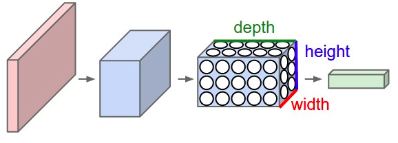
In comparison with regular neural networks, the different layers of a CNN have the neurons arranged in three dimensions: width, height and depth. Further due to the spatial architecture of of CNNs, the neurons in a layer are only connected to a local region of the layer that comes before it. Normally, the neurons in a regular neural network are connected in a fully-connected manner. Finally the output layer of a CNN reduces the images into a single vector of class scores, that are arranged along the depth dimension.
In the following the different layers that a CNN inherits are examined to gain further insight.
Convolutional Layers
The conv layer is the core building block of a CNN that does most of the computational heavy lifting. The conv layer reads an input, such as a 2D image or a 1D signal using a kernel that reads in small segments at a time and steps across the entire input field. Each read results in an interpretation of the input that is projected onto a filter map and represents an interpretation of the input.

The figure above is an example of a conv operation in 2D, but in reality convolutions are performed in 3D. Let’s explain how is the Conv network performed. First of all the convolution is performed on the input volume with using of a filter to then produce a feature map. During the execution of the convolutional, the filter slides over the input and at every location a matrix multiplication is performed and sums the results onto the feature map. The area of our filter is also called the receptive field and the size of it is 7x20.
Pooling Layer
The pooling layer follows the convolutional layer, in which the aim is dimension reduction. The reason is that training a model can take a large amount of time, due to the excessive data size. The pooling layer represents a solution to this issue. For example one can consider the use of max pooling, in which only the most activated neurons are considered. Moreover, pooling does not affect the depth dimension of the input image. However, the reduction in size leads to a loss of information, referred to as down-sampling. Nonetheless, pooling enables a decrease in computational power for the following layers and also works against overfitting.
Further, pooling can be used to extract rotational and position invariant feature extraction, as max pooling, as stated before preserves only the dominant feature value. Thus, the extracted dominant feature is potentially from any position inside the region.
Activation function
An activation function is f(x) is important to make the network more powerful and add ability to it to learn something complex and complicated from data. The CNN calculates the weighted sum of its input, adds a bias and then decides it should be activated or not. A neuron is calculated:
Y = ∑(weight * input) + bias
The value of Y can be ranging from –inf to +inf. By adding the activation function the output of neural network will be determined and the resulting values will be mapped between 0 to 1.
The Activation function can be basically divided into 2 types:
- Linear Activation Function
- Non-Linear Activation Functions
Linear Activation Function
As you can see the function is linear and the functions will not be confined between any range. F(x) = x As range the linear function has –infinity to infinity and it doesn’t help with the complexity of usual data that is fed to the neural networks.
Non-linear activation function
The Non-linear Activation Functions are the most used activation functions. It makes it easy for the model to generalize or adapt with variety of data and to differentiate between the output.
Also another important feature of a Non linear Activation function is that it should be differentiable. It means that the slope(the change in y-axis and x-axis) isn’t constant.
For our model we used the Relu (Rectified Linear Unit) function.The ReLu is the most used activation function in the world.Since, it is used in almost all the convolutional neural networks or deep learning.
Relu function
We use the ReLu activation function in our approach, as the function returns 0 if it receives any negative input, but for any positive value x it returns that value back. It can be written as: F(x)0 max(0,max)
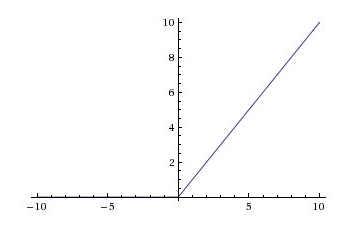
As you can see the ReLu function is simple and can allow our model to account for non-linearities and interactions. In the following it is described how ReLu captures Interactions and Non-linearities:
Interactions
Example: Let’s say we have a neural network with a single node. For simplicity, we assume it has two inputs A and B. The wights from A and B into our node are 2 and 3 respectively. So the output is f(2A + 3B). We use the ReLu function four our f. An output we’ll have 2A+3B if our f positiv, otherwise the output value of our value is 0, if our f in negative.
No-linearities
A function is non-linear if the slope isn’t constant. That means, that the ReLu function is non-linear around 0, but the slope is always either 0 (for negative values) or 1 (for positive values). As we saw before a Bias is important to calculate the weight of the neuron.
Example: Let’s consider a node with a single input called A, and a bias. If the bias term takes a value of 7, then the code output is (7+A). If A is less than -7, the output is 0 and the slope is 0. If A is greater than -7, then the node’s output is 7+A, and the slope is 1. So the bias term allows us to move where the slope changes. So far, it still appears we can have only two different slopes. Real models have many nodes. Each node can have a different value for it’s bias, so each node can change slope at different values for our input.
Fully-connected Layer
The last layer within a CNN is usually the fully-connected layer that tries to map the 3-dimensional activation volume into a class probability distribution. Further, it is to mention that the fully-connected layer is structured like a regular neural network. Therefore, an activation function, in our case ReLu, is used to activate the output to map it to sales value.
Summary of layers
As we described above, a CNN can be thought of as a sequence of layers, in which every layer of the CNN transforms the input volume of activations to another layer through a differentiable function. Therefore, three main types of layer to build a CNNs architecture can be identified, namely: Convolutional layer, Pooling Layer and Fully-Connected Layer.
In summary:
- The simplest CNN architecture is a list of layers which consequently transform the input image into an output image
- Distinct types of Layers are CONV/FC/RELU/POOL
- Moreover the layers accept an input 3D volume, which is transformed into an output 3D volume
- The layers consist of parameters (e.g. CONV/FC do, but RELU/POOL do not)
- Certain layers potentially have additional hyperparameters (e.g. CONV/FC/POOL do, RELU doesn’t)
Why CNN and not TCN
We want to identify key differences with respect to Temporal Convolutional Networks (TCNs). The term Temporal Convolutional Networks is a vague term that could represent a wide range of network architectures. The differentiate of the characteristics of TCNs are:
- Causality of the architecture (no information from future to past)
- Mapping any sequence of any length to an output sequence of the same length.
- In other words the TCNs do is simply stacking a number of residual blocks together to get the receptive field that we desire.
Shaojie Bai, J. Zico Kolter, and Vladlen Koltun (2018) also provide this useful list of advantages and disadvantages of TCNs.
- TCN‘s provides a massive parallelism and short both training and evaluation cycle.
- Lower memory requirement for training, especially in the case of long input sequences.
- TCNs offer more flexibility in changing its receptive field size, principally by stacking more convolutional layers, using larger dilation factors, or increasing filter size. This offers better control of the model’s memory size.
However, the researchers note that TCNs may not be as easy to adapt to transfer learning as regular CNN applications because different domains can have different requirements on the amount of history the model needs in order to predict. Hence, when transferring a model from a domain where only little memory is needed to a domain where much longer memory is required, the TCN may perform poorly for not having a sufficiently large receptive field. Therefore we are using in this blog the CNN application to predict the daily sales for the Rossman stores. An important secondary benefit of using CNNs is that they can support multiple 1D inputs in order to make a prediction. This is useful if the multi-step output sequence is a function of more than one input sequence. This can be achieved using two different model configurations. Multiple Input Channels: This is where each input sequence is read as a separate channel. Multiple Input Heads: This is where each input sequence is read by a different CNN sub-model and the internal representations are combined before being interpreted and used to make a prediction.
Technical Considerations
The biggest difficulty related to the architecture of a CNN that needs to be noted is the memory bottleneck. Ultimately, most modern GPUs have a 3/4/6GB memory limit. This results in the following main source of memory, which should be considered. First, the intermediate volume sizes that describe the number of activations at each level of the CNN, plus their gradients. Normally, this is where most of the activations are located. These activations are retained because they are needed for backpropagation. However, it is possible to reduce this through an intelligent implementation, as long as a CNN only executes the current activations at the given test time and stores them at any level. Previous activations are then stored at the lower level. Also of consideration are the parameter sizes, as these contain the numbers holding the network parameters and their gradients during back propagation. If the network does not fit, it is possible to reduce the batch size, where most of the memory is normally consumed by the activations.
Installing packages
In this step we install the required packages in order to build our CNN. The keras library helps us build our convolutional neural network. Further, import a sequential model which is a pre-built keras model in which we were able to add the layers. Therefore, we import the convolution and pooling layers and also import dense layers. The dense layers are used to predict the labels. Thereafter, the dropout layer reduces overfitting and the flatten layer expands a three-dimensional vector into a one-dimensional vector.
Data Preparation
CNNs are used to process image data and, as such, their input data need to be understandable as a set of images. Images are usually stored as two- or three-dimensional matrices where the first two dimensions determine the shape of the object itself and the third dimension holds information about the colour of the specific image - each color is created out of combination of red, green, and blue (RGB), therefore this third dimension holds a number describing the shade of each particular particular color.
The data table describing the revenues of various Rossmann stores looks like an image in no way. Therefore, an important step in our model building is going to be modifying data so that they can be understood as an image. From a table like this
, we want to construct an images based on this or better to say, a set of such images.
Data set contains no missing values and problems with encoding, thus we proceed to ordering it so that days describing the same store are logically after each other, then to eliminating, redundant data, such as day of month, etc. and other variables which can be constructed using other variables. It is also very important to recode the categorical variables into so-called One Hot Encoding. It is type of encoding typically used in Machine Learning which creates a dummy variable for each value of the original variable, so for example in the case of day of the week variable, it creates variables for day1, day2, and so on and then puts 1s where valid. Using one variable with various numeric levels would detriment the neural network because in the algebraic operations connected to weight-updating (and gradient descent), the categories associated with higher numerical values would have a higher numerical effect (higher importance) in calculations.
We can further eliminate variables Store and as the id of the store does not interest us, Date is important until we come to reshaping part, however after that, we can also get rid of this variable.
An example of an image we created from the dataset is presented in the following.
<img style=” width:500px;display:block;margin:0 auto;“src=”/blog/img/seminar/CNN/image_1.png">
Tensors
Tensor in the world of machine learning is understood as a multidimensional array of data. It is a generalisation of the concept of a matrix. It has an order which describes the number of its dimensions, where, for example a scalar is a tensor of the zeroth order, a vector is a tensor of the first order, a matrix a tensor of the third order. For higher orders there are no generally known names. This understanding of a tensor is different, simpler and not to be confused with the purely mathematical definition of tensor mainly used in physics and engineering. (Tensor Decomp and Applications). In that case, tensor is a multidimensional array obeying certain transformation laws under the change of coordinates - and this second part of the definition can lead to differences in understanding what is and is not a tensor. (In case of interest in tensor algebra, see Supervised tensor learning) The notion of tensor in machine learning is, therefore, quite simple and we will construct it as a 4 dimensional numpy array where the first dimension describes the number of images, the second and third the number of dimensions of each image and the fourth the color depth. To simplify our model, we will work only with the shades of grey, thus the fourth dimension is of size 1. This makes it irrelevant, however we still need it to create a four-dimensional tensor because the function for convolutional layer Conv2D in Keras expects one dimension for the color specification of the pixel, thus 3-dimensional tensor for each image.
Constructing this 4-dimensional process out of our original data frame is a multiple-stage process. First of all, we need to consider what we are going to model. Our goal is not the same as the goal of the competition. We will be predicting one day after a 90-day period. We used only stores which had complete data. These formed a great share of the total amount which spared us work with missing values. There were 934 such stores, each store containing a 942-days-long time series. The maximum possible amount of 91-day periods (because we need also the following day as a label) is 852, which is constructed by rolling the time frame over the whole time series of one store. This gives us the total amount of 795,768 time series which we can model. The rolling window approach solves also the problems which could arise if we decided to model specific months or quarters and distinguish between them such as different lengths of time frames. In that case we would have to modify images to the same size using for example cropping, centering, n crops, or padding.
Final Dataset
Also, we did not work with all possible time series which we got. To save some computing-power and time consumption we used only 5,000 time series for training. As a validation set, 20% of these were extracted and the final model was evaluated on 500 new test time series. These steps should significantly help us in evading overfitting.
Explain the reshaping process
On our way to getting 4D tensor, the method reshape connected to data frames in pandas came very handy. We needed to have all the info (all variables together with the day) in one row. This is easily done in two-step procedure as follows
Now we have a data structure which we need, although another small change will be needed for the final neural network algorithm. This, however, shall be discussed later.
Example of modeling artificial data with CNN
To get a small glimpse on how CNNs actually perform and how much we can expect from them we created a set of 3 types of time series, which we tried to predict using firstly, time series analysis (arima models) and then a simple convolutional neural network. The first time series is a sine-like function, where the values oscillate (some noise is created by adding normally distributed value) around 5 for Monday, 10 for Tuesday, and 15, 15, 10, 5 for following days with Sunday having always value 0 as the stores are closed. 91-days long time series were created such that each time the time series started on a random day (so it could be shifted) however it always followed this simple rule (so if the time series starts with Sunday it would start with 0, continue with 5, and so on).
The second type of time series was a function which we called a strong_poor trend. This is a time series with some characteristics of a random walk. Sunday was assigned again value 0. Other days would have values oscillating around 10 and in each week there was a day where the value of sales spiked to 35 and on the following day returned to almost zero (exception is if the spike happens on Saturday, then 0 follows). The third type of time series was created from these two, such that it changed randomly the type after one week. All three can be seen in the following figure.
For our time series analysis we used R language with package forecast, as this was faster and it was not our aim to show such an analysis in Python. For each type, we took a set of 1,000 time series and modelled each one (except for type one, where because of periodicity one model was good enough) by an arima model estimated automatically by the package. We then looked at the Mean Absolute Error (This was the only measure which we could right away compare to results from our NN without any other programming).
We can see that the sine-like function can be modelled pretty well and the predicted values are very close to the real ones. However, it is not able to precisely predict zeros.
The sine-like arima models can be still improved by first extracting the sine trend and then we get even better results. In case of type two and three, the results are dramatically worse. It can be expected that the spikes cannot actually be predicted because they are pseudo-random, however, a good model could learn that after such a great value a value close to zero follows. The arima models, however, are not able to do this. Also, as the third type is even more random even worse, although the difference between type two and three is not great.
Followingly, we trained a neural network on these three time series. The sine-like time series was so easy for the CNN to learn that with 2 convolutional layers, batch size 5, 300 hundred neurons, filter 7*1 and stride 7, it learn it almost perfectly with MAE 0.0012. To our surprise it actually learnt to predict 0 precisely and so the error can be considered to be systematic, because some randomness is introduced in the original trend. Other results can be seen in the table, however, the network gave us significantly better results in general.
An interesting observation is, that the best results in type two and three were given by kernels of size 7*1 (one week) and stride 42, which was a randomly chosen number without any time significance. We first hypothesised that because of the high level of randomness present in the time series, it would be beneficial for the model to increase the kernel size. However, this did not prove to be true. The stride 42 probably better filters our various short trends which are present in the data and helps the model to learn too much of the current time series. 3 convolutional layers did not bring much improvement.
To conclude, convolutional neural networks are very strong in predicting regular trends and perform also better when the trends are more random. As the sales can partially show regular trends and irregularities could be encrypted in other variables (of which the final CNN will make use) we assume CNN will be much more powerful in predicting the sales. With this assumption and basic idea of which parameterization of CNN worked best on simple data, we went on to build the final model.
Final CNN model
Here after the code for your final CNN model is presented.
Summary & Results
To summarize, the results of our CNN model can be derived in the following.
print(model.evaluate(x_test,y_test))
print(model.metrics_names)

#batch size 500 epochs 50 unit 300
#1 layer 5677.9359 MAE

#batch size 250, epochs 30, units 300
#1 layer 5677.9359

#batch size 50, epochs 30, units 300
#1 layer 5677.9359

#batch size 500, epochs 30, units 300 kernel (7,1) !!!
#1 layer 790.93658

#great strides bring nothing
#batch size 500, epochs 80, units 300 kernel (7,1) , stride 7!!!
#1 layer 778.0873

#bs 250, epochs 76, unit 300, (14,1), stride 7
#1 layer 730.569597

#bs (smaller) improves the results
#bs 100, epochs 34, unit 300, (14,1), stride 7
#1 layer 741.61

#bs 100, epochs 34, unit 300, (14,1), stride 7
#1 layer 741.61

#bs 50, epochs 65 (25 patience), unit 300, (14,1), stride 7
#1 layer 726

#kernel size seems to b pretty decisive

#bs 50, epochs 100 (25 patience), unit 300, (21,1), stride 7
#1 layer 729.57215

#bs 50, epochs 94 (25 patience), unit 300, (21,1), stride 7
#1 layer 719.2241

#bs 200, epochs 100 (25 patience), unit 300, (14,20)!!!, stride 7
#1 layer 709.901245

#bs 200, epochs 178 (100 patience), unit 300, (14,20)!!!, stride 7
#1 layer 713.1515

#batch size 500 epochs 50 unit 300
#2 layers 782.8316 MAE


500/500 [==============================] - 8s 15ms/step
[782.831650390625, 782.831650390625]
['loss', 'mean_absolute_error']
From the results we can conclude that kernel size played an imporant role with respect to the prediciton of sales. We found out empiricaly that the best length of kernel is 14, which represents the time period of two weeks. Also, to our surprise the kernel of size (7x1) delivered similar results to a kernel size (7x20), although this kernel does not take into account more complex relations between the features.
The number of neurons of 300 proved to be the best choice even with respect to this complex problem. In addition we tested different batch sizes and epochs to achieve even better results, however, these parameters did not influence the results as much as we thought. Another approach we used was to add more layers to our CNN model, this did not have the effect we wanted to achieve, but instead increased computational time highly.
The benchmark model, which we took into account, estimated following days of 500 same test time series (although without taking into account other features except sales), using some seperate automatically estimated ARIMA models for each time series. The derived mean absolute error from the benchmark model was 2.629,253.
References
-
Convolutional Neural Networks, Arden Dertat , 08 November 2017 https://towardsdatascience.com/applied-deep-learning-part-4-convolutional-neural-networks-584bc134c1e2
-
An intuitive guide to Convolutional Neural Network, Daphne Cornelisse, 24 April 2018 https://medium.freecodecamp.org/an-intuitive-guide-to-convolutional-neural-networks-260c2de0a050
-
An Empirical Evaluation of Generic Convolutional and Recurrent Networks for Sequence Modeling, Shaojie Bai, J. Zico Kolter, Vladlen Koltun,19 Apr 2018
-
https://www.kaggle.com/dansbecker/rectified-linear-units-relu-in-deep-learning
-
How to Develop Convolutional Neural Networks for Multi-Step Time Series Forecasting,Jason Brownlee, 8 october 2018 https://machinelearningmastery.com/how-to-develop-convolutional-neural-networks-for-multi-step-time-series-forecasting/
-
Convolutional Neural Networks from the ground up https://towardsdatascience.com/convolutional-neural-networks-from-the-ground-up-c67bb41454e1
-
CS231n Convolutional Neural Networks for Visual Recognition http://cs231n.github.io/convolutional-networks/#conv
-
Tensor Decompositions and Applications, Tamara G. Kolda & Brett W. Bader