Neural Networks into Production

Authors: Mahdi Bayat, Denis Augusto Pinto Maciel, Roman Proskalovich

Motivation

Training and tuning machine learning model is a hard task. There are many variables involved that can make or break your results. However, also very important is, after fine tuning your model, to be able to deploy it, so it can be accessed by other researchers, developers and applications.

A very common way to accomplish that is by using an API.

Use Case

As a data scientist, you will need to interact with other professionals that don’t have the same expertise that you have when it comes to quantitative models. They will be very interested in the predictions your models are able to deliver, but not so much in the technicalities it involves.

Imagine you work for a fashion online shop and are faced with the task of creating a model to predict which clothes are likely to fit the customer’s body. You get as input whole-body pictures of some customers and their purchase history. You decide to tackle the problem using deep learning and mange to create a very good model. After some discussion, the management level of your company decides that the results are good enough and that they want to offer this new feature on their online shop. The workflow of the app is simple: the customer uploads a picture of herself and receives a suggestions stemming from your algorithm.

To you, this means the model, which has run so far on your machine, needs to be deployed to a server and be accessible to the whole application. Most likely the frontend part of the online shop will receive the image uploaded by the customer and send its pixels to your model. The frontend developer is not interested in how pixels turn into prediction. She merely wants to send the picture and get back the IDs of the suggested products, so they can be displayed.

Considering everything, you decide to build an API. Here we will walk you through the process of deploying a deep learning model via an API. Instead of customer’s pictures, we will use handwritten digits and employ the model to predict what digit it is. And instead of a frontend mobile application, an R session will be querying the API and consuming the predictions.

Reproducibility with Conda Environments

It’s good practice to create a Conda environment to train and later deploy our model. By doing that, a fresh version of Python is installed. It will only have access to the packages you explicitly install while in the environment. This has some advantages:

• you won’t fall into the gotchas of depending on a package you have previously installed and have forgotten to install on the server. With a simple command, you can get a snapshot of all the packages used in an environment.
• your results can easily be shared with and reproduced by other researchers.
• you have direct control over the versions of your package. Different environments can have different of packages. Often models require different versions of packages (or even of Python itself) to run properly. This way you are free from the burden of uninstalling and reinstalling specific versions of a package depending on the project you want to work on.
• it reduces the size of the application, when putting it to production. You will only install the strictly necessary packages to run the model. Packages you might have installed for other projects and are present in the global installation of Python, won’t be installed.

Creating new environments

Our environment will be called dl-in-production. It will use Python version 3.6.4 and we install the packages keras, pandas and flask. To do that, run the following command:

conda create --name dl-in-production python=3.6.4 keras flask jupyter pandas

After doing that, you will be presented with the list of dependencies which need also to be installed. Agree to install them by typing yes and the installation will begin.

After few minutes, our newly created environment should be ready to use. To enter it, run the command below if you are using macOS or Linux:

source activate dl-in-production

For Windows users, the command must be the:

activate dl-in-production

To make sure you are using a complete independent version of Python, run the commands:

which python
python --version

You will see that Python’s binary inside the dl-in-production environment is in a different path than the global installation. In my case, it’s in ~/miniconda3/envs/dl-in-production/bin/python. And the version is exactly the one we specified when creating the environment: Python 3.6.4.

Installing extra packages

Not all packages must be installed at once. If you find out you need to install an extra package to your environment, make sure you have activated environment and run the command below. The package will be available to usage.

conda install <package-name>

In fact, there is one extra package, we need to install to be able to use our freshly installed version of Python from within a Jupyter notebook. The nb_conda package is very handy and makes possible to choose pick every single environment you have created from within a Jupyter notebook without having to leave it.

conda install nb_conda

After starting a notebook, go to Kernel > Change kernel in the menu and choose the Kernel of your like.

Conda environments is a very rich utility. We have only scratched its surface so far. Further details on how to create and manage environments can be found here.

Sharing your environment

Once you are done with your model and want to share it with others or want to install all the necessary packages to run it on a server, you can take a snapshot of the environment by running:

conda list --export > requirements.txt

This will save the list of all the packages available in dl-in-production to requirements.txt. Now you can share the code together with requirements.txt and the only thing your audience needs to do to recreate your environment is to create a brand new environment on their machine by running the conda create command and passing the requirements file as an argument.

conda create --name dl-in-prodution --file requirements.txt

Training the model

The model we will deploy was trained using Keras. All the steps taken to build it are documented in this jupyter notebook. It’s important to know that we saved the model in the model.h5 file.

Building an API

We will deploy our model with Flask. Flask is a lightweight web framework written in Python. But before deploying our real model, we will create a toy application, so the reader can have a quick glimpse at how Flask works.

Toy App

To create our very first Flask app, copy and paste the following code into a file and name it toy-app.py.

from flask import Flask

app = Flask(__name__)


@app.route('/')
def hello():
    return 'Hello World!'


@app.route('/another-greeting')
def hi_there():
    return 'Hi there!'


@app.route('/square/<number>')
def square(number):
    number = float(number)
    return f"The square of {number} is {number**2}"

Then got to the terminal and run:

FLASK_APP=toy-app.py flask run

The command will spin up a server on your machine and you will be able to access it though your browser by going to this URL http://localhost:5000/. That’s it. We have implemented our first application. Our mini web application has three endpoints that can be accessed with any browser. You can go to:

• http://localhost:5000/ and receive a nice Hello World! or to
• http://localhost:5000/another-greeting if you prefer a “Hi there!” instead or to
• http://localhost:5000/square/15 and discover that 15 squared equals 225.

As you can see, our API not only renders static pages but can receive and process inputs from the client such as the number 15 we passed to the square/<number> endpoint. In fact, any client capable of sending HTTP requests can interact with our application. You can even do that via the command line using curl. Try running the following commands:

curl http://localhost:5000/square/99

Real App

Awesome. Now that we have an app running and got a first grasp of how Flask works, we can adapt the structure of the code to make it serve our deep learning model.

It takes around 30 lines of code to create an Flask app that serves our model:

from flask import Flask, jsonify, request
from keras.models import load_model
import numpy as np

app = Flask(__name__)

model = load_model('model.h5')


@app.route('/home', methods=['GET'])
def home():
    return """
    Hi! This is a Flask app.
    You can get some predictions by hitting the /predictions endpoint.
    """


@app.route('/predict', methods=['POST'])
def predict():
    # get all the data passed by the client in the request
    data_client = request.get_json()

    input_data = data_client['input']

    input_array = np.array(input_data, dtype=float)/255
    out = model.predict(input_array)
    out = np.ndarray.tolist(out)

    return jsonify(out)


if __name__ == 'main':
    app.run(port=8080, debug=True)

First, the necessary packages are imported and a Flask app object is instantiated. Also, the trained model is loaded to memory. The model, which was saved in the model.h5 file, is now available across the Flask application and can be called from anywhere to deliver its predictions.

Our API has two endpoints:

• /home tells you what the app is about. It is included there, so we can rapidly test if the most basically functionalities are working correctly once we try to deploy the model.
• /prediction is where the magic really happens and we will go through it in detail.

The first thing to notice is that the method for this endpoint is POST instead of GET. This is necessary since the prediciton endpoint is expecting to receive the image’s pixels as JSON in the body of the request. The correct way to it is to make a POST request according to HTTP.

Once the endpoint is activated by an incoming request, it calls the get_json function from Flask’s request submodule and transforms the JSON body of the request into a Python dictionary. Our API was designed in such a way that it expects the data to be passed in a field called input. In case we were to make our API available to the public, this should definitely be documented, so other developers know how to pass the data. The next step is to isolate the input and transform it into a numpy array.

    data_client = request.get_json()
    input_data = data_client['input']
    input_array = np.array(input_data, dtype=float)/255

Then, we run the predictions on the received data, transform it into a list, transform the list to JSON and finally send it back to the client in the response.

    out = model.predict(input_array)
    out = np.ndarray.tolist(out)

    return jsonify(out)

That’s it. We have just written a fully functioning API and we are ready to test it. First, let’s spin it up by running:

export FLASK_APP=app.py
flask run

Test if the app’s basic functionalities by going to http://localhost:5000/home. Did you get the expected message? Does everything work fine?

Let’s then test the core function of our API, namely the prediction endpoint. To do that, we will use R. It doesn’t matter which tool we use to test our API. It could as well be a React app written in JavaScript making the requests (which would likely be the case in the fashion online shop example above). What is important to notice is that our API is capable of communicating with any application that can send HTTP requests. We chose R here because it is likely that data scientist will have some familiarity with it.

This is the code we will use to test the prediction endpoint of our API.

library(httr)
library(tidyverse)

# Read in the MNIST test dataset
test <- read_csv("./data/mnist_test.csv", col_names = FALSE)

# Rename the first column to name and add id
test <- test %>%
  rename(labels = X1) %>%
  mutate(ids = 1:nrow(.)) %>%
  select(ids, labels, everything())

# Pick one digit and sample n_samples of it to get prediction for
digit <- 2L
n_samples <- 500

test_filtered <- test %>%
  filter(labels == digit) %>%
  sample_n(n_samples)

ids <- test_filtered$ids
labels <- test_filtered$labels

features <- test_filtered %>%
  select(matches("X\\d{1,3}")) %>%
  as.matrix()

body <- list(input = features)
r <- httr::POST("http://localhost:5000/predict",
                body = body,
                encode = "json")
r_content <- content(r)

prediction_prob <- r_content %>%
  map(~ unlist(.x)) %>%
  unlist()

df <- data_frame(
  prediction_prob,
  digit,
  ids = ids %>%
    map(~ rep(.x, 10)) %>%
    unlist()
  ) %>%
  group_by(ids) %>%
  mutate(
    is_max_prob = prediction_prob == max(prediction_prob),
    pred_label = as.integer(row_number() - 1)
  ) %>%
  ungroup()

Let’s go through the code to understand what it is doing. First, we need to load the MNIST test dataset into R and slightly transform it. We add an id column and rename the label column from X1 to labels.

Then we filter some observations to get predictions for. Here we chose 500 images of the digit 2 to send to the API. We are sending only the pixel values for each picture. Labels and ids are kept out, since the model is neither allowed to see the digits – that’s the whole point of the prediction – nor is it expecting to have a label or id column in the request body. The features matrix is the data we are going to send over.

# Pick one digit and sample n_samples of it to get prediction for
digit <- 2L
n_samples <- 500

test_filtered <- test %>%
  filter(labels == digit) %>%
  sample_n(n_samples)

ids <- test_filtered$ids
labels <- test_filtered$labels

features <- test_filtered %>%
  select(matches("X\\d{1,3}")) %>%
  as.matrix()

The httr package makes it very simple to send HTTP requests. We wrap the feature matrix in a named list under the input field, which is the field in the request body our API is expecting to find the data. We use the POST function and pass “json” to the encode argument. httr converts out data automatically from a list to JSON and sends it over to the API.

The API processes the request and send back a prediction, which is stored in a response object r. We can access the response sent by the API by applying the content function to it.

The response came back as JSON and was automatically transformed into a hairy, nested R list. Some data wrangling is necessary to finally get to a vector of probabilities. The vector has 10 entries for each observation, each entry corresponds to the probability associated to one of the nine possible digits.

body <- list(input = features)
r <- httr::POST("http://localhost:5000/predict",
                body = body,
                encode = "json")
r_content <- content(r)

prediction_prob <- r_content %>%
  map(~ unlist(.x)) %>%
  unlist()

We construct a dataframe to have predicted probabilities, ids and real digit label all in one place.

df <- data_frame(
  prediction_prob,
  digit,
  ids = ids %>%
    map(~ rep(.x, 10)) %>%
    unlist()
  ) %>%
  group_by(ids) %>%
  mutate(
    is_max_prob = prediction_prob == max(prediction_prob),
    pred_label = as.integer(row_number() - 1)
  ) %>%
  ungroup()

We are finally able to inspect how good a predictor our deployed model is. From the 500 digits, 492 were correctly classified as 2.

df %>%
  filter(is_max_prob) %>%
  mutate(is_correct_prediction = digit == pred_label) %>%
  pull(is_correct_prediction) %>%
  table()

# FALSE  TRUE
#     8   492

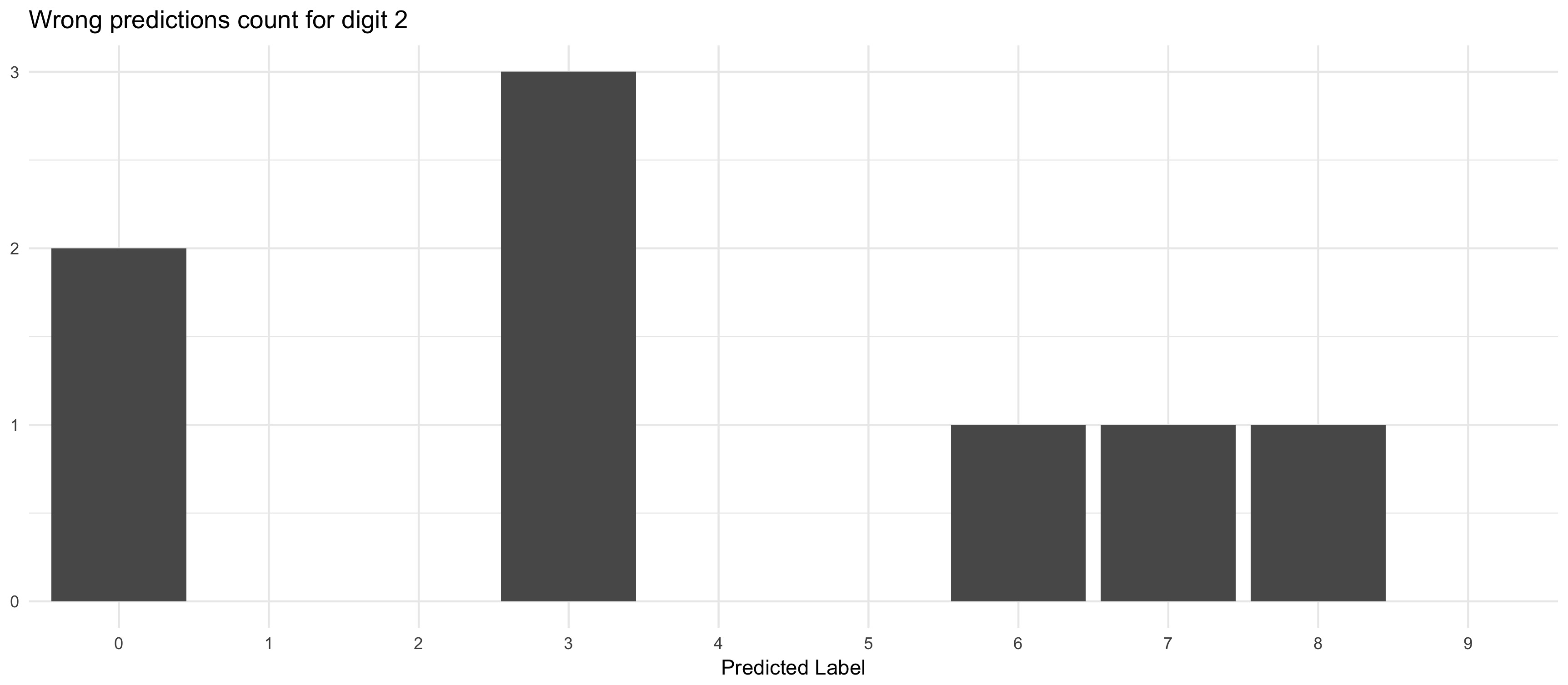
Three times has our model labelled a 2 as a 3 and twice as a 0. The plot below shows how the 2s were misclassified.

p <- df %>%
  filter(is_max_prob) %>%
  count(pred_label) %>%
  filter(n != max(n)) %>%
  mutate(pred_label = factor(pred_label, levels = 0:9)) %>%
  ggplot(aes(x = pred_label, y = n)) +
  geom_col() +
  scale_x_discrete(drop = FALSE) +
  labs(title = glue::glue("Wrong predictions count for digit {digit}"),
       y = NULL,
       x = "Predicted Label") +
  theme_minimal()
p

Deploy to Heroku

We are finally ready for the last step: deploy our API on the web so anyone with an Internet connection can have access to it.

There are many options on the market to accomplish that. We chose to use Heroku here because it is very simple and it allows us to deploy our API for free (at least until it reaches a certain limit of resource consumption).

You will have to create a Heroku account if you still want to follow along. After creating the account, you will be able to log to your Heroku dashboard and from there you can create a new Heroku app. We have named our app flask-digit-classifier.

The way the deployment will is the following:

• we will create a git repository in the folder we have our application
• set an upstream branch a link it to Heroku’s CLI
• commit and push the necessary files to run the app to the upstream branch and let Heroku do the hard lifting.

Thus, you will also need to install:

• git
• Heroku Command Line Interface

After installing Heroku CLI, login with the credentials of your newly created account by running:

heroku login

We also need to explicit tell Heroku what our dependencies are. Before creating requeriments.txt, there is one extra package we need to install in order to deploy our model. gunicorn will be our HTTP server, because its more suitable to production environment than Flask’s builtin option.

pip install gunicorn
pip freeze > requirements.txt

We will use pip to replicate our local Python environment on the server. At the time of the writing, you cannot install via pip the nb_conda package that was used in order for us to have access via Jupyter notebook to the various conda environments. So we need to exclude them from our requirements.txt, otherwise we get an error. Remove from requirements.txt the following lines:

nb-conda==2.2.1
nb-conda-kernels==2.1.0

We need now to create the Procfile file with instructions to Heroku on how to deploy our app. Create a new file called Procfile (make sure not to add any extensions such as .txt to it) and write the single line below in it:

web: gunicorn app:app

We are ready to transform our folder into a git repository and set Heroku as a remote repository.

git init
heroku git:remote -a flask-digit-classifier

We can finally add and commit the necessary files to run our API. A refresher on the content and function of each file:

• app.py contains our Flask API.
• model.h5 contains our trained model that will be loaded by the Flask app.
• requirements.txt contains the list of the packages needed for our API to run.
• Procfile contains instructions on how Heroku should deploy our app.

That’s it. Add and commit the files and push it to Heroku’s remote branch.

git add Procfile app.py model.h5 requirements.txt
git commit -m 'initial commit'
git push --set-upstream heroku master

The files will be uploaded and the application deployed. You can follow the status of the deployment in the command line or in the browser with Heroku’s dashboard.

In our case, our app was deployed to https://flask-digit-classifier.herokuapp.com/. You can run all the test we implemented before (both with the browser and with R) simply by changing http://localhost:5000/ for your newly deployed app’s URL.

Shiny App

Whew! We hope you made thus far. As a surprise we have developed a slightly more sophisticated client for our API. We created a Shiny App to help you visualize how the model makes its predictions and where it falls short.

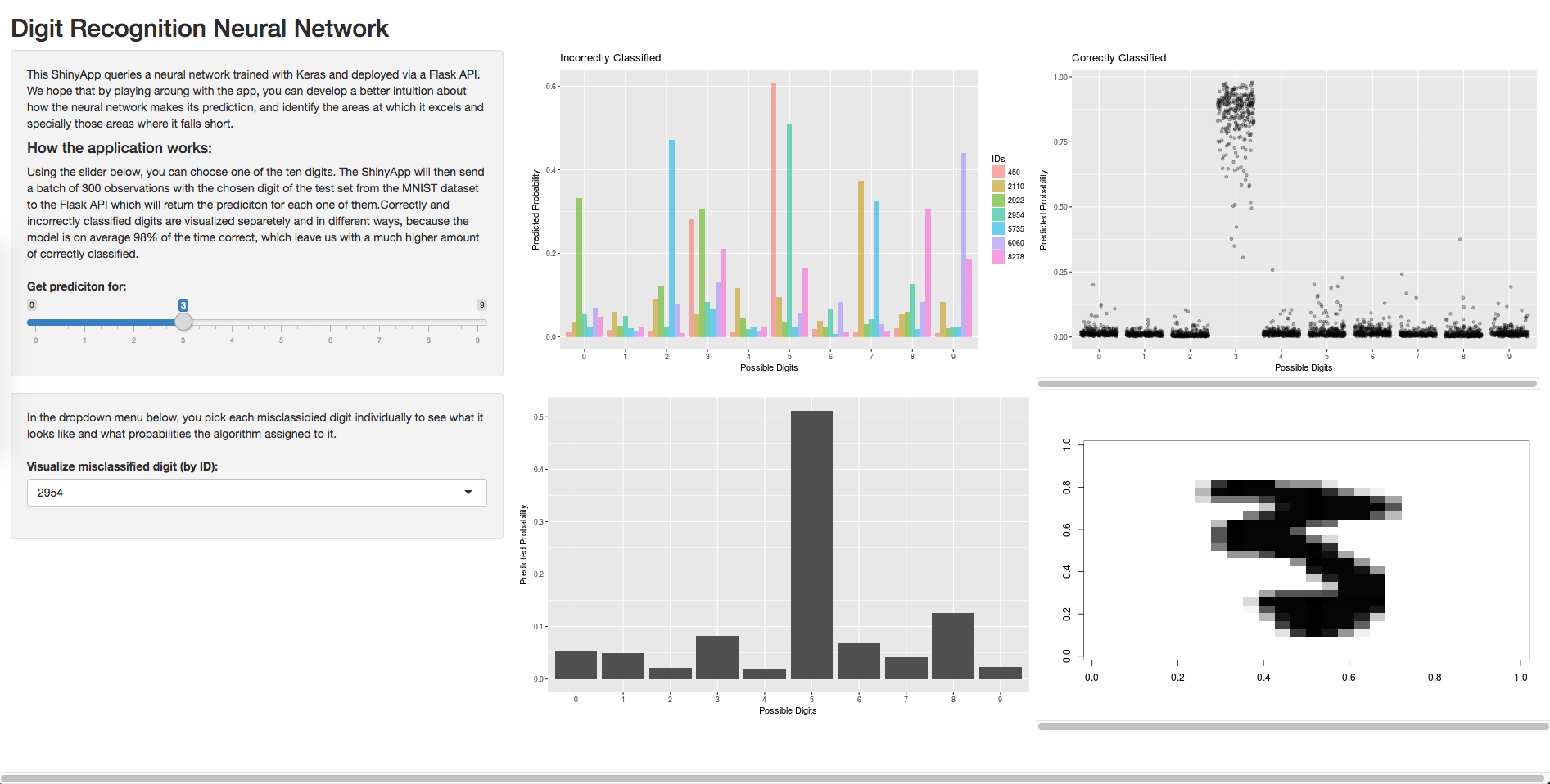
Here you have links for:

• Shiny App: https://denismaciel.shinyapps.io/digit-classification
• Flask API: https://flask-digit-classifier.herokuapp.com/home

The API sending the predictions is exactly the same one we just built and deployed to Heroku. The Shiny App is deployed on a completely different platform and is communicating with the Flask API over the Internet. Quite neat, right?

If you got lost somewhere along the way, you can find all the code used here in the following repository:

• https://github.com/denismaciel/foundations-of-deep-learning

We hope this tutorial has helped you to deploy your very own deep learning model! If anything’s still unclear, don’t hesitate to get in touch. Drop us a line at denispmaciel@gmail.com.