Financial Time Series Predicting with Long Short-Term Memory

Authors: Daniel Binsfeld, David Alexander Fradin, Malte Leuschner

Introduction

Failing to forecast the weather can get us wet in the rain, failing to predict stock prices can cause a loss of money and so can an incorrect prediction of a patient’s medical condition lead to health impairments or to decease. However, relying on multiple information sources, using powerful machines and complex algorithms brought us to a point where the prediction error is as little as it has ever been before.

In this blog, we are going to demystify the state-of-the-art technique for predicting financial time series: a neural network called Long Short-Term Memory (LSTM).

Since every new deep learning problem requires a different treatment, this tutorial begins with a simple 1-layer setup in Keras. Then, in a step-by-step approach we explain the most important parameters of LSTM that are available for model fine-tuning. In the end, we present a more comprehensive multivariate showcase of a prediction problem which adopts Google trends as a second source of information, autoencoders and stacked LSTM layers built to predict share price returns of a major German listed company.

Since this blog post is designed to introduce the reader to the implementation of LSTMs in Keras, we will not go into mathematical and theoretical details here. We can highly recommend and suggest the excellent blogposts by Colah and Kapur (more advanced) to pick up the theoretical framework on LSTMs in general before going through this blogpost.

To bridge the theoretical gap, we just want to briefly explain why LSTMs should be applied for time series prediction as state-of-the-art machine learning technique.

Short Intuition on LSTM architecture

Proposed by Hochreiter and Schmidhuber in 1997, LSTMs provide a solution to the so-called vanishing gradient problem faced by standard recurrent neural networks (RNN). LSTMs are a type of RNNs, so they have the same basic structure. However, the extension of LSTMs is that the LSTM-cell itself (which is part of a recurrent neural network) is a much more extensive series of matrix operations. Ultimately, this advanced version allows the model to learn long-term dependencies by introducing a new kind of state, the LSTM cell state. Instead of computing each hidden state as a direct function of only inputs and other hidden states, LSTMs compute it as a function of the cell state’s value at that time step. The following illustration gives a graphical explanation of LSTMs.

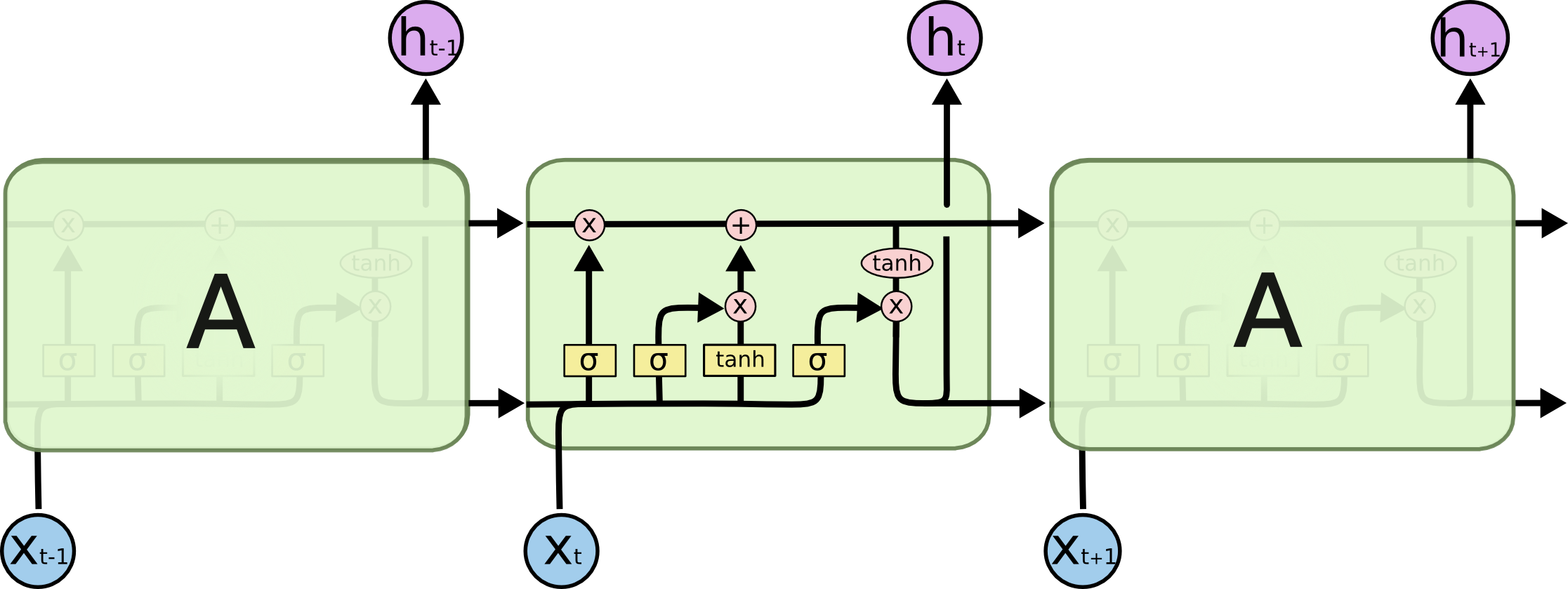Figure from: Colah’s Blog

The cell state is the top line in the LSTM cell illustrated in the figure above. It can be intuitively thought of as being a conveyor belt which carries long-term memory. Mathematically, it is just a vector. The reason to use this analogy is because information can flow through a cell very easily without the need for the cell state being modified at all. With RNNs, each hidden state takes all the information from before and fully transforms it by applying a function over it. Each component of the hidden state is modified according to the new information at each single time step. In contrast, the LSTM cell state takes information and only selectively modifies it while the existing information flows through. This methodology solves the vanishing gradient problem. Why? The key is that new information is added, i.e. not multiplied, to the cell state. Different to multiplication in RNNs, addition distributes gradients equally, the chain-rule does not apply. Thus, when we inject a gradient at the end, it will easily flow back all the way to the beginning without the problem to vanish. But enough theory, let’s get our hands dirty with the implementation in Keras.

Getting started…

Data Collection

Before we can start our journey we would like to introduce two useful APIs that can make your life a lot easier:

• Pandas_datareader can be used to download finance data via the Yahoo Finance API. You can see a small snipped down below. Include your stock and your time frame. API does normally not provide returns, which are commonly used in practice. We added another line that calculate log returns for your. Log returns are great! Check it out: Here is a good Google trend API.

• Pytrends can access the reference. In the second box you can find a more comprehensive example that collects data from Google, loops the code, and can even continue downloading at another day (your daily quota is unfortunately limited). Please have a look at the code. If you spend a moment, we are sure you can figure it out. For more information: Here is a good reference. The details of the snipped are not to important for our modelling, but have a look!

# Get Yahoo Data
import pandas_datareader as pdr

stock = pdr.get_data_yahoo(symbols='#your stock ticker', start=datetime(2012, 1, 1), end=datetime(2017, 12, 31))
stock = stock['Adj Close'] # or one of the other columns (i.e., opening prices, Volumes)
stock_returns = np.log(stock/stock.shift())[1:] #calculate log returns

# Download Data from google Trends
from pytrends.request import TrendReq
import datetime
import os
google_username = #(...) #INCLUDE YOUR GOOGLE ACCOUNT
google_password = #(...)
pytrend = TrendReq(google_username, google_password, custom_useragent="My Pytrends Script")

formatter = "{:02d}".format

databegin = list(map(formatter, range(0, 19, 3))) #change TIME here.
dataend   = list(map(formatter, range(4, 25, 3))) #downloads for hourly data atm

lastdate = datetime.date(2018, 3, 12) # Until when do you want to download

file = open("daysleft.txt")
daysprior = int(file.read())
file.close()

while daysprior>2:

    file = open("daysleft.txt", "w")
    file.write(str(daysprior))
    file.close()

    daysbefore = lastdate - datetime.timedelta(days=daysprior)

    keywords = ["Volkswagen"] #INCLUDE KEYWORDS HERE!
    for i in range(0, len(databegin)):
        begin = daysbefore.strftime("%Y-%m-%d") + "T" + databegin[i]
        end   = daysbefore.strftime("%Y-%m-%d") + "T" + dataend[i]

        timeframestring = begin + " " + end

        for j in range (0, len(keywords)):
            pytrend.build_payload(kw_list=[keywords[j]], timeframe=timeframestring)
            df = pytrend.interest_over_time()
            df.to_csv("../data/" + keywords[j] + "/" + timeframestring + ".csv")

    begin = daysbefore.strftime("%Y-%m-%d") + "T21"
    end   = (lastdate - datetime.timedelta(days=daysprior - 1)).strftime("%Y-%m-%d") + "T01"
    timeframestring = begin + " " + end
    for j in range (0, len(keywords)):
        pytrend.build_payload(kw_list=[keywords[j]], timeframe=timeframestring)
        df = pytrend.interest_over_time()
        df.to_csv("../data/" + keywords[j] + "/" + timeframestring + ".csv")

    daysprior = daysprior -1

This should just give you an idea on where to start. If you work with financial data, these should come in handy. We are now going to use a dataset that is already prepared to showcase sequence modelling with Keras. The data was collected from the same APIs, you just learnt about. Our dataset has 7 columns, combining finance data from Yahoo and query data from Google:

• date represents trading days between 2012 and 2017.

• googLVL represents an index on how much “Volkswagen” was googled.

• volLVL represents the total Volume traded for that specific day.

• dif_highlowLVL represents the difference between the day’s highest and lowest stock price. You can think of it as proxy for volatility.

• googRET represents the log returns of googLVLs.

• daxRET represents the log returns of the DAX. It is a proxy for the market movements.

• y_closeRET represents our target variable as a log return. It is the closing price for the Volkswagen AG stock for the specified date. We are using the closing and not the adjusted closing price because it is reasonable to assume that dividends and market split information are also represented in the Google signal (As a reminder: Adjusted closing prices are corrected for financial events, i.e. stock splits or dividend payments).

We are using everything except date. We could also try to extract further features like dummies or a seasonal effect. We save that for next time. Our data should incorporate some seasonal effects already. Nevertheless, be creative!

Download the data sheet (final_df_VW.CSV)

# We read in the dataset
data = read_csv("final_df_VW.csv")
data = data.iloc[:,1] # delete column you dont want to use for training here!
                      # We are deleteting date here.

Data Preprocessing

We are left with our six variables including our target. Before we start with our model training we need two more steps. First, we include a MinMaxScaler from the sklearn package. It always makes sense to think about proper preprocessing such as normalization. If we included the dataset without it, volLVL could completely dominate our traning and skew our model. It often makes sense if your features are on a similar scale. Please see below the function for the normalization. Notice that we also save the scaler, we are using! You can use it for example to reverse the scaling after your predictions. The second step is a little more involved but it is crucial for working with sequences in Keras.

# function to normalize
def normalize(df):
    """
        Uses minMax scaler on data to normalize. Important especially for Volume and google_lvl
        @param df: data frame with all features
    """
    df = DataFrame(df)
    df.dropna(inplace = True)
    df = df.values
    df = df.astype('float32')
    scaler = MinMaxScaler(feature_range=(-1, 1))
    norm = scaler.fit_transform(df)
    return scaler, norm

Keras

Before we get into the exciting part, a small introduction…

“Keras is a high-level neural networks API, written in Python and capable of running on top of TensorFlow, CNTK, or Theano. It was developed with a focus on enabling fast experimentation. Being able to go from idea to result with the least possible delay is key to doing good research.” (Keras Documentation)

Our examples use Keras with Python 3.5, running TensorFlow as a backend. We will build a small LSTM architecture to teach you the in and outs of Keras’ sequence modelling. At this point, we expect you to understand what a recurrsive layer does and how it is special. We will talk about hidden states and weight updates, truncated backpropagation, and other things. If all that is new to you, check out some of the very detailed blogs we recommended in the ‘theory’ part. There are many other blogs and examples which go rather slowly. Jason Brownlee’s blog covers many ideas slowly for beginners. This blog does try to provide a condensed application example, that does not only showcase the easiest one-to-one prediction. If you just came here accidentally without any idea of Keras the 30s guide can bring you up to speed. For more involved file an issue to the Keras’ Github. Most of the time they are happy to help!

A little more preprocessing…

The most confusing thing for people starting to work with Keras’ recurrent layers is getting used to the shape of the input matrix. In contrast to a standard Multilayer perceptron, recurrent networks’ input has an additional dimension.

• The input matrix is 3D, where the first dimension is the number of samples in your batch (denoted as batch_size). You can think of it as the number of rows of your input data after which you want your weights to be updated (careful: weights are not states). A higher batch_size reduces your computational time by reducing the number of updates. In many cases, especially if you are short on training data, you would set this to one and just update your weights after every sample. We will do that for our stock prediction, since we only end up with about 1500 training days. If you had a different use case (i.e., Natural Language Processing) it could be beneficial to update weights only every 5 samples (i.e., batch_size = 5).

• The second dimension represents the new time domain (timesteps). Timesteps define the number of steps in the past you are unfolding your recurrent layer. They define where the backpropagation is truncated to. It is important to understand that the longer your sequence per sample is (more timesteps) the more computationally expensive your optimization gets, since the gradient is computed for every defined timestep. If you are used to auto-regressive statistical modelling techniques, timesteps are difficult to understand. In a standard feed forward neural network (FFNN) or i.e. ARIMA setup, it would be natural to include your timesteps (lags) as features. Here is where many people struggle. In LSTM, the right way to handle time dependencies is in the second dimension. For stock market prediction, it is crucial to find well defined time dependencies. If we set this to i.e. seven, every feature would backpropagate one week, with 30 - one month etc. Technically, it is also possible to include different features with different timesteps. Missing steps would be padded with 0. Would that be a problem? Most likely not, since the model should learn to ignore them.

• The last dimension represents features. There are six in our stock price example if we want to include the target variable also as a feature.
  

Now that you understand the batch_input_shape (batch_size, timesteps, features) of a recurrent layer, you might have noticed that our dataset does not really have the correct dimensions to be fed into the model. Below you can see the function which solves this. The idea is simple: We shift the input and append the new column to our dataset. Thus we extend the dataset according to our specified timesteps.

# Append with timesteps
def createTimeSteps(df, lags=1):
    """
        creates the amount of timesteps from the target and appends to df.
        How many lags do we use to predict the target.
        @param df: data frame with all features
        @param lags: number of lags from the target that are appended
    """
    df = DataFrame(df)
    columns = list()
    for i in range(lags, 0, -1):
        columns.append(df.shift(i))
    columns.append(df) #add original
    # combine
    output = pd.concat(columns, axis=1)
    # replace rows with NaN values
    output.fillna(0, inplace = True)
    return output

Now we’re good to go. We are using our loaded dataset from above, apply normalize, extend by our timesteps, split into training and test set with TRAINING_DAYS, choose our features and our target y. It is good practive to define CONSTANTS in capital letter in the beginning of your training. It helps you to keep eveything structured and is very convenient for testing different setups.

# Everything prepared...
scaler, normalized_data = normalize(data)

BATCH_SIZE = 1 # batch size during training
TS = 14 # length of Sequence we use for our samples (7 = week, 30 = month)
FEATURES = 6 # number of features in data set
TRAINING_DAYS = 1250 # Training/Test split for data

full_df = createTimeSteps(normalized_data, TS)
full_df = full_df.values # Training vs Test

train = full_df[:TRAINING_DAYS, :]
test = full_df[TRAINING_DAYS:, :]

input_var = int(TS*FEATURES) # Every feature has as many columns as defined timestep
target = -1 # Our Volkswagen AG stock price is the last column of our dataset
X_train, y_train = train[:, :input_var], train[:, target]
X_test, y_test = test[:, :input_var], test[:, target]

X_train = X_train.reshape(TRAINING_DAYS, TS, FEATURES)
X_test = X_test.reshape(X_test.shape[0], TS, FEATURES)

Model Design

Similar to any Keras network we can design recurrent architectures. Just add an LSTM layer instead of a normal dense layer. If you call the function, make sure that your input dimensions fit our dataset. Otherwise you will not be able to train your model.

Our first model is kept simple, but in case you do not know anything about Keras, please refer to the Keras in 30s guide. This should give us a starting point to explain different concepts and extensions.

# Our first very easy model
def helloModel(timesteps, features, batch_size=1):
    model = Sequential()
    model.add(LSTM(16, input_shape=(timesteps, features)))
    model.add(Dense(1))
    model.add(Activation('linear'))  
    model.compile(loss='mse', optimizer='adam', metrics=['mse'])  
    return model

Our helloModel has only one layer with 16 hidden neurons. It passes its input to the dense layer which produces a one-step-ahead forecast. The first extention we would like to introduce is return_sequence:

• In Keras when return_sequence = False: The input matrix of the first LSTM layer of dimension (nb_samples, timesteps, features) will produce an output of shape (nb_samples, 16), and only output the result of the last timesteps training.

• In Keras when return_sequence = True: The output shape for such a layer will also be 3D (nb_samples, timesteps, features) since an output is saved after every timesteps. This allows us to extend our model in two different ways. First, we can start stacking LSTM layers, since every previous LSTM layer also produces a 3D output. Additionally, we can also make the model predict many-to-many. If we specify return_sequence = True for the last layer it will produce 3D predictions (Careful: If you would like to apply another layer to every timesteps and not only to the last one, you need to use a TimeDistributed wrapper).

# Our return model
def returnModel(timesteps, features, batch_size=1, return_sequence = False):
    model = Sequential()
    model.add(LSTM(32, input_shape=(timesteps, features), return_sequence = True ))
    model.add(LSTM(16, input_shape=(timesteps, features), return_sequence = True ))
    model.add(LSTM(8, input_shape=(timesteps, features), return_sequence = return_sequence ))
    if return_sequence:
        model.add(Dense(1))
    else:
        model.add(TimeDistributed(Dense(1)))
    model.add(Activation('linear'))  
    model.compile(loss='mse', optimizer='adam', metrics=['mse'])  
    return model

We are stacking three different LSTM layers and included the option to predict many-to-many, applying a final Dense layer to every timesteps. We still have to be careful here since our target y should be a matrix now. If we extend y by the same timesteps as our input matrix, you can think of the prediction as a many-to-many lagged by one each.

The last architecture we are presenting is inspired by a research paper of Bao et. al (2017). It is a simplified version but has similar perks. We use it to introduce three more concepts before we can release you into the wild world of sequence modelling:

• A single Auto-Encoder precedes the three stacked LSTM layers. The auto-encoder is introduced in order to denoise the data and to extract the most common features from an unsupervised dataset. The sequence-to-sequence auto-encoder uses a bottle neck architecture, where four LSTM nodes are sandwiched by two eight node LSTM layers to reshuffle information in meaningful features. We can think of it as deep learning feature extraction.

• Furthermore, we introduce the stateful and shuffle parameter. If stateful = False, the hidden states of the LSTM neurons are reset after every batch. After the reset, states are reinitiated with 0. As an effect, batches are treated independently through time and not connected. If stateful = False, Keras does not require you to define batch_size within the first layer Input_shape= (timesteps, features). We can use that in training, when we believe that the timesteps we defined properly represents the length of time dependency and an independent training is reasonable. If we expect a longer time dependency to be useful we should use stateful = True. If stateful = True, states are propagated through batches and only reset manually (model.reset_state()). Using shuffle = True together with stateful = True will not make any sense, since the output destroys the ordering of the time series and produces pure chaos. Careful: It is important to think about the timing of the state reset. Common practice is resetting after every epoch. Without it, the model would treat every new epoch as an extension of the original time series and not as the same time series fed in again. In model training, Keras requires you to exactly define the input shape in the first layer only (batch_input_shape=(batch_size, timesteps, features)).

# create Bao Model
def bao2017(timesteps, features, batch_size=1,
            state_config = False, return_config = False):
    model = Sequential()

    #AUTOENCODER
    model.add(LSTM(input_dim=features, output_dim=8, return_sequences=False))
    model.add(RepeatVector(4))
    model.add(LSTM(output_dim=8, return_sequences=True))
    model.add(TimeDistributed(Dense(features)))
    model.add(Activation('linear'))

    #STACKED MODEL
    if state_config:
        model.add(LSTM(128, batch_input_shape=(batch_size, timesteps, features),
                       return_sequences=True, stateful=True))
    else:
        model.add(LSTM(128, input_shape=(timesteps, features),
                       return_sequences=True, stateful=False))
    model.add(LSTM(64, return_sequences=True, stateful=state_config))
    model.add(LSTM(32, return_sequences=return_config, stateful=state_config))
    #... add more layers
    if return_config:
        model.add(TimeDistributed(Dense(1)))
    else:
        model.add(Dense(1)) #not 1 but 'features' if many-to-many   
    model.compile(loss='mse', optimizer='adam', metrics=['mse'])  
    return model
    

The number of hidden neurons is somehow arbitrary. We could also include different ones but this is the setup used by Bao et. al (2017). It is important for the auto-encoder to have the sandwich architecture (8 to 8 neurons). We haven’t really touched on the RepeatVector layer, but it does essentially what it says (Check the Keras RepeatVector documentation for more).

What is left to do? We have the data, we have the models… let fit! Our last function does that for us. We can specify the number of our model, data, epochs, batch_size, if we want our states to be reset per batch by state_config, and decide if we would like shuffle to the True. We set model.reset_state in a way that is resets after every epoch, and saves the training results in two list.

# Fit the model
def fitting(model, X, y, val_X, val_y, epochs, batch_size=1, state_config=False, sf=False):
    """
        fits the model to the data via keras API.
        @param model: before designed model setup
        @param X: correctly reshaped input data
        @param y: correctly reshaped target
        @param val_X, val_y: correctly reshaped test data
        @param epochs: number of epochs to repeat training
        @param batch_size: number of rows after the weights of the network are updated
        @param state_config: True/False - if true, model is trained with stateful mode and
        states are resetted every epoch
        @param sf: True/False - shuffle mode. If stateless, this makes sense to increase
        generalization of the model
    """
    if state_config:
        training_mse = list()
        val_mse = list()
        for i in range(epochs):
            model.reset_states()
            result = model.fit(X, y, batch_size=batch_size, epochs=1, validation_data=(val_X, val_y), shuffle=sf)
            training_mse.append(result.history['mean_squared_error'])
            val_mse.append(result.history['val_mean_squared_error'])
    else:
        result = model.fit(X, y, batch_size=batch_size,
                        epochs=epochs, validation_data=(val_X, val_y), shuffle=sf)
        training_mse = result.history['mean_squared_error']
        val_mse = result.history['val_mean_squared_error']


    return result, training_mse, val_mse

Sit through, we are almost there! Put it together and get your predictions:

# Almost forgot... your libraries
import keras
from keras import Sequential
from keras.models import load_model
from keras.models import Sequential
from keras.layers import Dense, Activation, LSTM, Dropout, TimeDistributed, RepeatVector

from sklearn.preprocessing import MinMaxScaler

import pandas_datareader as pdr
from pandas import read_csv, DataFrame
import pandas as pd

from datetime import datetime
import numpy as np
import matplotlib.pyplot as plt
import os

# Our new CONSTANTS
EPOCHS = 30 # number of training Epochs
STATEFUL = True # stateless/stateful
SF = False # activate shuffle
RETURN_SEQ = False # many to many prediction (outputs results of every TS)

# Choose a model
model =  bao2017(TS, FEATURES, batch_size=BATCH_SIZE,
                state_config = STATEFUL, return_config = RETURN_SEQ)
# Fit the model
result, training_mse, val_mse = fitting(model, X_train, y_train, X_test, y_test, EPOCHS, batch_size=BATCH_SIZE,
                state_config=STATEFUL, sf=SF)
# Predict the model
yhat = model.predict(X_test, batch_size = BATCH_SIZE)
print(yhat.shape)
print(y_test.shape)

# Plot the model
plt.plot(y_test, label='y')
plt.plot(yhat1, label='yhat')
plt.legend()
plt.show()

plt.plot(training_mse, label='Training: MSE')
plt.plot(val_mse, label='Test: MSE')
plt.legend()
plt.show()

That was hard work! As a wise economist once said, …