Sentiment Analysis using Deep Learning

Authors: Katja Metzger, Aydin Sader Fosalaie, Ninos Yonan

Outline

• Sentiment Analysis Introduction
  
  

• Case Study

  • Keras IMDB Dataset
    
    
  • Data Analysis
    
    
  • Word Embeddings
    
    
  • Convolutional Neural Network
    
    

• Summary

Sentiment Analysis Introduction

Sentiment analysis is a very beneficial approach to automate the classification of the polarity of a given text. A helpful indication to decide if the customers on amazon like a product or not is for example the star rating. The same applies to many other use cases. However, the underlying basis for the review rating is the raw text material containing the customer’s opinion. Therefore, analyzing and categorizing the sentiment of reviews, emails, blog posts and other texts is undoubtedly useful for firms to evaluate the perception of their customers regarding their products, services or as well of the firm by itself. Analyzing the public opinion and brand awareness supports managing the strategy of a firm and the business decisions.

Now before we start with the our tutorial, let’s first have a look on the basic sentiment analysis steps and characteristics.

Sentiment Analysis

• Computational study of opinions, sentiments and emotions in text
• Task: Classifying the expressed opinion of a text (positive, negative, neutral)
• Sentiment analysis uses:
  • natural language processing (NLP)
  • text analysis
  • computational techniques
• to automate the extraction or classification of sentiment from text

Different levels of Sentiment Analysis:

• Document based: One score for the whole document (e.g. review)
• Sentence based: Does sentence express positive, neutral, negative opinion
• Aspect based: Focus on a specific aspect and identify what people like/dislike

Why do we need sentiment analysis?

• it becomes a hot area in decisionmaking
• 97% of customer’s read online reviews for local business in 2017 (Local Consumer Review Survey 2017)
• 85% of consumers trust online reviews as much as personal recommendations (Local Consumer Review Survey 2017)

Challenges of Sentiment Analysis

• abbreviations (e.g. LOL, YOLO, CD9 → Code 9, parents around)
• emoticons
• sarcasm
• negation

Preprocessing

Example

1. Step Tokenization: Split each token/word for itself

2. Step Stop word removal: remove stop words such as: by, my, and, a…

3. Step Stemming: reduce each token/word into the original word stem/root form

4. Step Sentiment assignment: assign positive, negative and neutral words and the overall sentiment

Case Study:

Keras IMDB Movie Review Dataset

For this tutorial, we chose the so called Large Movie Review Dataset often referred to as Keras IMDB dataset. Starting with the procedure of the data exploration, we will further explain how to devise a model that can predict the sentiment of movie reviews as either negative or positive. Therefore, we will use Python and the Keras deep learning library. However, the overall goal of this tutorial is to focus on explaining how all the things work rather than achieving the best accuracies. Our models perfomed good but might have also achieved better accuracy results when using a bigger dataset.

Keras IMDB Movie Review Dataset

• The dataset has originally been used in Maas et al. (2011): Learning Word Vectors for Sentiment Analysis
• Overall distribution of labels is balanced
  • 50.000 reviews (25.000 for training and 25.000 for testing with each 12.500 reviews marked as positive or negative)
• It is a binary (0 = negative or 1 = positive) classification problem.
  • The negative reviews have a score from 4 out of 10,
  • The positive reviews have a score from 7 out of 10.
  • Thus, neutral rated reviews are not included in the train/test sets.
  • To not bias the ratings between the movies, in the entire dataset, not more than 30 reviews for a specific movie were allowed.
• The reviews have been preprocessed and encoded as a sequence of integer word indexes, where each word is indexed by its overall frequency (e.g. integer “5” encodes the 5th most frequent words in the dataset).

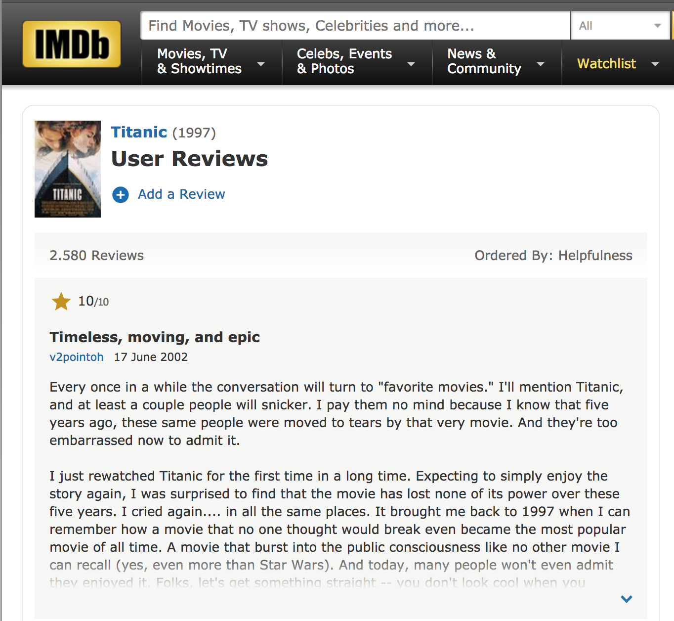Source: http://www.imdb.com/title/tt0120338/reviews

Tutorial:

• The overall goal and focus is to evaluate whether sentiment expressed in movie reviews obtained from IMDB can effectively indicate public opinion
• The underlying data mining question becomes whether we can devise a model that can measure the polarity of the text accurately
  
  

Before we will have look into the Keras IMDB dataset and its characteristics you should keep the following assumptions in mind:

Movie reviews are not expected to have the same text length (number of words) Neural networks are expecting a fixed size of input vector We will therefore have to either truncate long reviews or pad short reviews Before building the deep learning models it is necessary to gain a clear understanding of the shape and complexity of the dataset. Therefore we show you how to calculate some crucial properties and how to find key statistics through data exploration. This is required because some of the following decisions taken when building the models were based on specific characteristics of the Keras IMDB dataset.

Now let’s have a deeper look at our data.

As you can see, we have 25.000 train and 25.000 test sequences.
Further, by printing the number of unique classes, it becomes obvious that it is a binary classification problem for positive and negative sentiment in the review.
The reviews consists of list of integers. Each integer represents one word in a movie review, where each word is indexed by its overall frequency in the dataset.

The top 10 most frequently used words across the dataset:

To show the top 10 most frequent words across the dataset we need to run the snippet below. Our helperfunction-file includes a function to load the IMDB dataset that contains the original reviews with their text. You can also download the original files here (https://s3.amazonaws.com/text-datasets/imdb_full.pkl). However, the most frequent words in the reviews are as expected the typical stopwords (“the”, “and”, “a”, “of”…).

Wordcloud

This wordclound illustration presents the most common words across the dataset but excludes the stopwords.
The most common words are: ‘movie’, ‘film’, ‘story’, ‘character’, ‘scene’…

If you look closer you will find also the terms ‘good’ and ‘bad’ within the wordcloud. In general, these words do not provide us with detailed information on the polarity of the reviews. Consequently, further exploration regarding the positive and negative sentiment words is needed.

Summary Statistics:

As you can see the number of unique words in the dataset is given as 88.585. This is an interesting fact indicating that there are less than 100.000 words within the whole dataset. Moreover, the calculated average review length amounts to 238.71 words in total with a standard deviation of 176.49 words.

Boxplot

As a result, we get to the information that most reviews have less than 500 words and the mass of the distribution can be covered with a length of 400 to 500 words. Further, the overall distribution review length is positively skewed.

Which words make a review positive or negative?

In addition, to show how the combination of words can influence the polarity of a given text, we need to have a basic understanding of the concept of n-grams. N-grams are the result of fragmenting a text into N consecutive pieces.

For example: “Good” (unigram) is definitely positive and “very good” (bigram) even more. However, “not good” (bigram) seems to be less positive.

Therefore, you can use the NLTK library to remove the stopwords from the original dataset. Further, you can apply a simple logistic regression to get more insights to what important unigrams and bigrams make a review positive or negative.

Which words make a review positive?

Which words make a review negative?

Which 2-grams make it positive?

Which 2-grams make it negative?

Word Embeddings

The Keras definition says that word embeddings turn positive integers (indexes) into dense vectors of fixed size. Generally speaking, word embeddings is a technique in the field of NLP. It describes a technique where words are encoded as dense vectors in a high-dimensional space that carry a meaning. Each word has a specific position within the vector space. This position is learned from the text during the training and is premised on the surrounding words. Training the model will cause that semantically similar words will appear closer together also in the vector space.

Bag of Words

A simple bag of words has for the same representation different meanings. Additionally, huge text datasets would be represented by a vector comprised by many zeros and only a few one’s which is not only inefficient but leads also to data sparsity.

• “Netflix is better than Maxdome”
  • Bag of words: [Netflix] [is] [better] [than] [Maxdome]
    
    
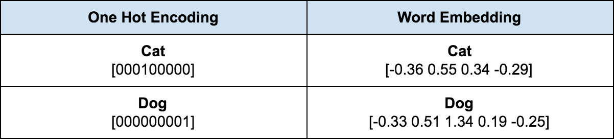
• One Hot Encoding: index of the specific word becomes a one, the rest becomes a zero
  • Maxdome → 00001
  • better → 00100
  • Netflix → 10000

One Hot Encoding - Problems:

1. Word ordering information is lost: * Netflix is better than Maxdome vs. Maxdome is better than Netflix * Different meaning but same representation
   
   

2. Data sparsity: * many zeros and few ones (imagine 20.000 zeros)
   
   

3. Words as atomic symbols * cat and dog would have the same distance as cat and apple * but cats and dogs are closer together (both are animals) * semantic similarity and relations is all learned from the data

4. Very hard to find higher level features when using One Hot Encoding
   
   

Example

Below we want to show you an example why using dense vectors has a computational benefit when working with deep learning models such as CNNs. First, imagine you have the sentence “deep learning is very deep”. Next, you have to decide on how long the vector should be (usually a length of 32 or 50). For this example we assign a length of 6 factors per index in this post to keep it readable.

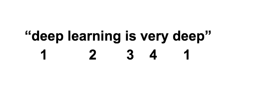
Now instead of ending up with huge one-hot encoded vectors, an embedding matrix keeps the size of a vector much smaller. The embedded vectors are learned during the training process. This is computationally efficient when using very big datasets. Below you see an example for the embedding matrix for the word deep:

deep = [.32, .02, .48, .21, .56, .15]

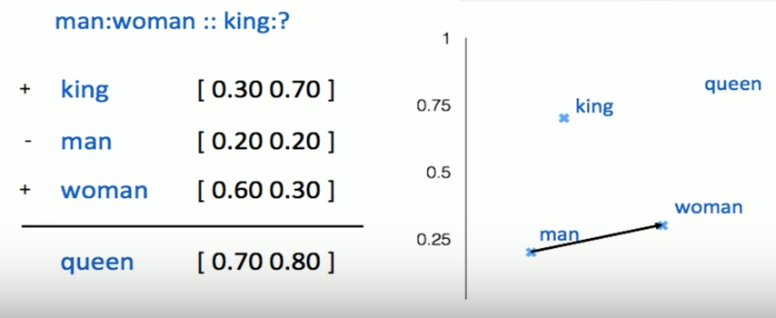
• Also relationships are learned, for example the information of gender
  
  
• Subtraction of vector [woman - man] is the same as [queen - king]

Word Embeddings - Benefits:

1. Trained in a completely unsupervised way, so you don’t need labeled data
   
   

2. Reduce data sparsity because you are not dealing with a huge number of 0/1 you have a lot of float values
   
   

3. Semantic hashing

   • representing the information of word meaning of the words
   • semantic hashing: semantically similar words are closer
     
     

4. Freely available for out of the box usage

Train Your Own Embedding Layer

In a Nutshell:

In the following you will see an example of how to learn a word embedding which is based on a neural network. This example aims to show how Keras supports word embeddings for deep learning in detail. First, it requires the input data to be integer encoded, so that each word is represented by a unique integer. Then the Embedding layer is initialized with random weights and will learn an embedding for all words in the training dataset. We will define a small problem with ten text documents and classify them as positive “1” or negative “0”. We are using a Keras Sequential Model to finish the task.

One Hot Encoding

Next, each document has to be integer encoded. This means that as input the Embedding layer will have sequences of integers. We use the Keras one_hot() function that creates a hash of each word as an efficient integer encoding. Further, the vocabulary size is estimated at 20.

Padding

As Neural Networks are expecting a fixed size of input vector we have to pad each document to ensure they are of the same length.

Keras Embedding Layer

Finally, we will define our Embedding layer as part of a neural network model for binary classification. The Embedding has a vocabulary of 20 words and an input length of 4 words. We will choose a typical embedding space of 8 dimensions. Importantly, the output from the Embedding layer will be 4 vectors of 32 dimensions each, one for each word. In the end, we flatten this to a one 32-element vector to pass on to the Dense output layer.

The trained model shows that it learned the training dataset perfectly (which is not surprising).

Machine Learning Approach for Sentiment Classification

In the following code section you will find our machine learning approach for the sentiment classification task on the Keras IMDB dataset.

First, we will load the dataset as done before. The input_dim describes the size of the vocabulary in the data. We used a vocabulary size of 5000 (0 - 4999). Overall, we tested the vocabulary size between 5.000 – 10.000 words to reduce the parameters and improve the performance. Second, for the output_dim (output dimension) we defined a 32 dimensional vector space in which the words will be embedded. Third, the input_lenght of the input sequences was set to 500 because we will only consider a maximum review length of 500 words, due to the distribution of review lengths seen in the boxplot in the data exploration part. As CNNs expect a fixed size of input vectors and we set the input_lenght to 500 words, we have to either truncate longer reviews or pad shorter reviews with zeros at the end when loading the data.

Multilayer Perceptron Model

One of the models we chose to predict the sentiment of the IMDB dataset is a multilayer perceptron model. It is a feedforward neural network. It consists of three layers, the input layer, the hidden layer and the output layer. It is interconnected over neurons, each of them is connected to the neurons in the next layer. We used a “Sequential” model from Keras to build the MLP. Keras defines this model as a linear stack of layers (Keras Documentation). The embedding layer which was built build already in the previous chapter Word Embeddings served as the input layer. The next step was to flatten this layer to one dimension and afterwards to add the hidden layer with 250 units. A rectifier activation function was used in this part of the model. The last layer has an output of one neuron which is binary and can have the values 0 or 1 (positive or negative). It is activated with the sigmoid function.

As you can see, this simple model achieved a score of nearly 87.38% which is very close to the original paper. But we can get more out of this. Therefore lets try another network model - the Convolutional Neural Networks.

CNN Model

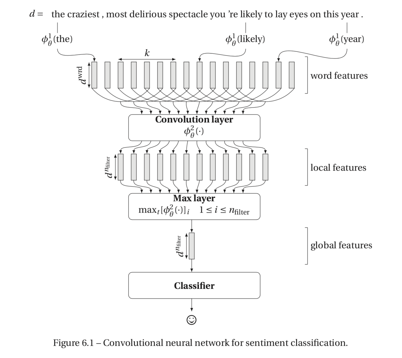
After performing a MLP, we conducted a one-dimensional convolutional neural network for the IMDB dataset. When looking at our dataset, an advantage for us is that Keras already provides the necessary one-dimensional convolutions as well as the Conv1D and MaxPooling1D classes. The first layer to start with is the embedding layer. After transforming the words into dense vectors they can be shifted to a convolutional layer, that with the help of the filters, indicates the proper sentiment in the sequence of words.

In contrast to image pixels, in which the filters in the convolutional layer would slide over local patches, in NLP tasks, the filters would instead slide over full rows of the input matrix representing the words. Therefore, the width of the filters is equal compared to the width of the matrix in the embedding layer. Nevertheless, the height may vary but it is quite common to determine a sliding window of over two to five words at a time.

Next, the pooling layer is applied right after the convolutional layer. Generally speaking, max-pooling is the most common implementation. An advantage of the pooling layer is the outcome of a fixed size output matrix. This process is inevitable because in the end the output has to be fed into the classifier. Furthermore, the operation aggregates features over a region by calculating the maximum value of the features in the region. This means that it reduces the output dimensionality while still keeping the most salient information.

Afterwards, the Flatten() operation takes the output and flattens the structure in order to create a single long feature vector, so that it can be used by the following dense layer for the final classification. The final dense layer with the activation function sigmoid transforms the output into a single output in order to indicate the sentiment.

In the end we used the binary_crossentropy loss function for our binary classification problem. Again, the Adam optimization algorithm is performed, since it is known to be very fast, efficient and had become very popular in recent deep learning model applications.

Source: https://infoscience.epfl.ch/record/221430/files/EPFL_TH7148.pdf

After two rounds we achieved quick a satisfactory outcome of 88.75% accuracy. Besides, it is an improvement compared to the end result of the MLP model we conducted earlier. Now there are a lot of opportunities to optimize and configure the model. You can play with the different settings and try to boost the performance.

Confusion Matrix

Calculating a confusion matrix can give you a better idea of what your classification model is getting right and what types of errors it is making. The confusion matrix below, visualizes the outcome of the binary classification:

• Total of 2813 wrong classifications and 22187 true classifications
• True negative: 11093 | False positive: 1407
• False negative: 1406 | True positive: 11094
• Accuracy: 88,75%

Summary

• In this tutorial, we discovered the topic of Sentiment Analysis with the Keras IMDB dataset.
  
  

• We learned how to develop deep learning models for sentiment analysis including:

  • How to handle the basic dictionary approach for sentiment analysis
    
    
  • How to load review and analyze the IMDB dataset within Keras
    
    
  • How to use and build word embeddings with the Keras Embedding Layer for deep learning
    
    
  • How to develop a one-dimensional CNN model for sentiment analysis and how it works for NLP
    
    

• How to continue with this tutorial?

  • Try to experiment with the number of features such as filter size in the convolutional layer
    
    
  • You can also experiment with several convolutional layers and maxpooling layers, etc.
    
    
  • Try to obtain higher accuracy

Limitations and further Topics

• CNNs are not able to encode long-range dependencies, and therefore, for some language modeling tasks, where long-distance dependence matters, other architectures are preferred:
  
  
  • Recurrent Neural Networks (RNN)
    
    
  • Long Short Term memory (LSTM)