Numeric representation of text documents: doc2vec how it works and how you implement it

Authors: Felix Idelberger, Alisa Kolesnikova, Jonathan Mühlenpfordt

Introduction

Natural language processing (NLP) received a lot of attention from academia and industry over the recent decade, benefiting from the introduction of new algorithms for processing the vast corpora of digitized text. A set of language modeling and feature learning techniques called word embeddings became increasingly popular for NLP tasks. Word2vec (Mikolov et al, 2013) became one of the most famous algorithms for word embeddings, offering a numeric representations of any word, followed by doc2vec (Le et al, 2014), which performed the same task for a paragraph or document.

The area of application is wide and encompasses online advertisement, automated translation, voice recognition, sentiment analysis, topic modeling and dialog agents like chat bots. Academia also received an efficient tool allowing to tap into the vast corpus of digital texts, from Shakespeare works to social media.

Regardless of the specific task at hand, its overarching goal is to obtain numeric representation of a document that reflects its content and, possibly, some latent semantic relationships within.New machine learning algorithms are often not well documented or miss in-depth explanation of the processes under the hood. One of the possible explanations suggests that many were developed by teams from technology companies like Facebook or Google, that would rather focus on application aspect. Doc2vec is no exception in this regard, however we believe that thorough understanding of the method is crucial for evaluation of results and comparison with other methods.

This blog post is dedicated to explaining the underlying processes of doc2vec algorithm using an empirical example of facebook posts of German political candidates, gathered during the year before elections to Bundestag.

We will start by providing some desciptive statistics of the dataset, followed with some theoretical backgound to embedding algorithms, in particular, word2vec’s SkipGram and doc2vec’s PV-DBOW, moving on to step-by-step implemetation in python, followed by the same actions performed using the gensim package. We will finish this blog by showing the application of the discussed methods on the political data, also touching vizualisation techniques.

Preparatory steps

In preparation for the following steps, we need to specify which packages to load and where we have stored the data:

Descriptive Statistics

The dataset consists of 177.307 Facebook posts from 1008 candidates and 7 major political parties who ran for the German Bundestag in the 2017 election. We collected all messages posted between 1 January and the election date on 24 September 2017, covering the entire campaigning period. The parties are included in order to later compare the candidates to them, but computationally they are treated no different then the candidates.

Sahra Wagenknecht, with a mean of 99.63 words per post, publishes quite long posts compared to Joachim Herrmann and Cem Özdemir who use on average less than half the amount of words in their posts.

Words per post by party: AfD and Die Linke candidates write longer posts on average than the candidates from the other parties.

A histogram of the words per post across all parties: A large majority of posts has less than 50 words

Theory

The goal of the empirical case study is to generate a concept space for each candidate, thus offering a visual representation of German political landscape. For this purpose we need an algorithm to construct an embedding layer that will contain the numeric representation of the semantic content of each candidate’s Facebook posts.

PV-DBOW is similar to the Skip-gram model for word vectors (Mikolov et al, 2013), we will revisit the word2vec algorithms to facilitate the methodological transition.

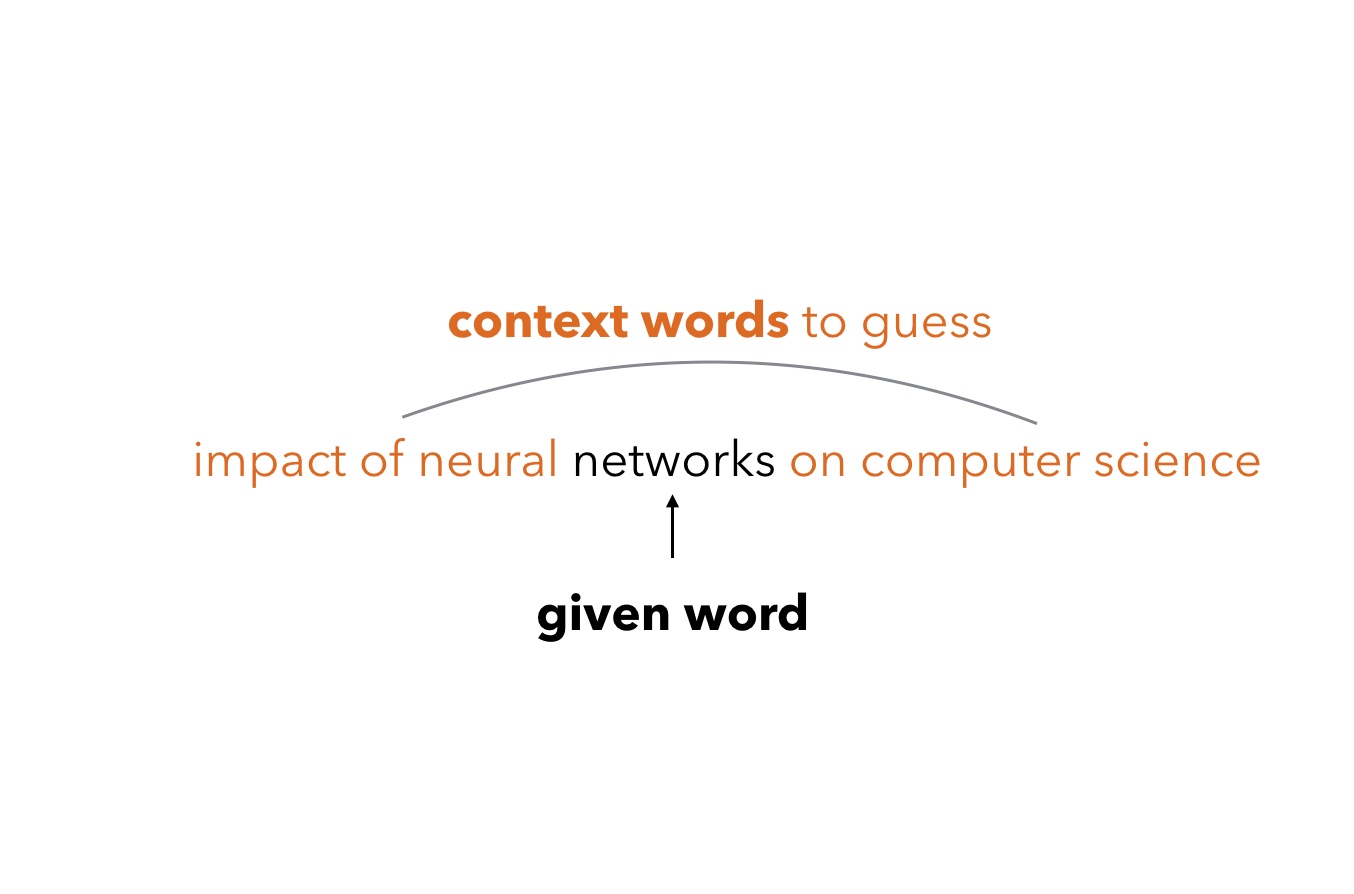
Word2vec is built around the notions of “context” and “target”. While CBOW predicts a target word from a given context, Skip-gram predicts the context around a given word. Using an example from our dataset, we would try to get “teilweise”, “laute”, “Gesetzentwurf” by giving “Diskussion” to the network (originally “teilweise laute Diskussion um den Gesetzentwurf”).

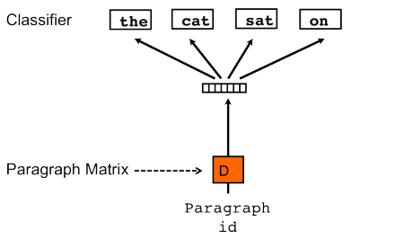
PV-DBOW performs a very similar task with the only difference of supplying a paragraph id instead of the target word and training a paragraph vector. Unlike PV-DM, PV-DBOW only derives embeddings for documents and does not store word embeddings.

Let’s try to train embedding vectors for each candidate in our dataset, using his or her facebook posts as one big text document.

Some preparation

We combined all the posts issued by the same candidate/party in order to obtain one document per candidate. By doing this, we ended up with 1015 text documents (1008 polititians and 7 parties) each containing the rhetorics of one candidate during campaigning.These paragraphs became the “docs” in our implementation of doc2vec and led us to giving the project the “candidate2vec” nickname. Each document is further tokenized in order to allow distinguishing individual words. Finally, we filter out stop words of the German language.

Some more preparation

A few more preparatory steps are required before the actual training: As a first step, a list of the m unique words appearing in the set of documents has to be compiled. This is called the vocabulary. Similarly, a list of of the documents is needed. In our case, these are the n aggregated corpora of Facebook posts of every candidate and the political parties.

For every training iteration, one document is sampled from the corpus and from that document, a word window or context is selected randomly.

In order to explain the internal structure, we need to get a clear understanding of the PV-DBOW workflow:

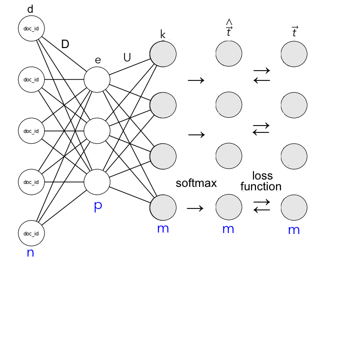
Input Layer

The input vector d is a one-hot encoded list of paragraph IDs of length n, with a node turning into 1 when the supplied ID matches the selected document.

Hidden layer

The hidden layer consists of a dense matrix D that projects the the document vector d into the embedding space of dimension p, which we set to 100. D thus has dimensions p__x__n and is initialized randomly in the the beginning before any training has taken place.

After the training, D will constitute a lookup matrix for the candidates, containing weights for the paragraph vector e (standing for embeddings). The latter will contain the estimated features of every document.

Output layer

In the output layer, the matrix U projects the paragraph vector e to the output activation vector k which contains m rows, representing the words in vocabulary. U has dimension m__x__p and is initialized randomly similar to D.

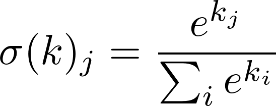
Softmax

The process of predicting the words from the context given the supplied paragraph ID is done through a multiclass classifier called softmax, which provides a probability distribution over the words for an input document.

k is then passed to the softmax function in order to obtain __t__^, the vector of the predicted probabilities of each word in the vocabulary to appear in the document

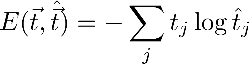
Backpropagation and cross-entropy

In the last step, the softmax probabilities t^ are compared with the actual words from the selected context. We can compute the cross entropy loss function, which sums up the products of the component-wise logarithm of t^ and the actual one-hot encoded vectors t. Since t is zero for the words outside the context, only the prediction error for the context word is taken into account.

The goal of the SGD is then to gradually reduce the loss function, minimizing the resulting difference with every iteration.

The gradients of the loss function on the matrices D and U will tell us how we need to update the weights that connect the neurons in order to reduce the loss function. They are obtained by taking the derivative of E with regard to the components of matrices D and U. For Skip-gram, \textcite{rong_word2vec_2014} shows how we need to update the weights by passing the prediction error back through the network, which cab be adapted to PV-DBOW as well. We therefore compute the output prediction error o of length m by substracting t from t^ and the error from the embedding layer h by projecting o into the embedding space by means of right-multiplying it onto U’.

The errors are computed for each of the c words in the given context and summed up before passing them back through the network. The sum of the output errors is right-multiplied with the transposed embedding vector e’ in order to obtain the update values for U, while the sum of the embedding-layer errors gets right-multiplied by d’. Before updating U and D, the updates are multiplied with learning rate alpha which limits how much the weights are adjusted at each step. A common choice is to start with alpha=0.025, gradually reducing it to 0.001.

The backpropagation concludes the training iteration for one document. Repeating these steps for all documents once would then constitute one epoch.

A note on efficiency

As running softmax on the whole vocabulary would be computationally inefficient, the following techniques are usually considered: hierarchical softmax (indexing the words in vocab) and negative sampling (output layer will contain correct words and only a bunch of incorrect ones to compare to).

Putting everythin in one loop

Here, we combine all the steps previously explained in order to complete the training for 1 epoch (or more if you want)

Visualisation with t-SNE

The paragraph vectors contain 100 components, which makes them hard to visualize and compare. A t-Distributed Stochastic Neighbor Embedding (t-SNE)(Maaten, 2008) is a popular technique for dimensionality reduction that is used widely in NLP. The concept follows the paradigm of visualizing similarities as proximity by minimizing an objective function that signifies discrepancies in the initial multidimensional format and final visual representation. Retention of information remains an obvious challenge when reducing the dimensions. t-SNE manages to preserve the clustering of similar components (unlike Principal Component Analysis, which focuses on preserving dissimilar components far apart). The algorithm assigns a probability-based similarity score to every point in high dimensional space, then performs a similar measurement in low dimensional space. Discrepancies between the actual and simplified representations are reflected in different probability scores and get minimized by applying SGD to the Kullback-Leibler divergence function, containing both scores (Kullback, 1951). The “t” in the name refers to the student distribution that is used instead of the Gaussian distribution when estimating probability scores, as the thicker tails allow to maintain larger distance between the dissimilar points during the score assignment, thus allowing to preserve local structure.

As we see, the simple model does not show any pattern among the candidates yet. In the following section, we use the python package gensim which allows run many more trining iterations in less time.

Application of doc2vec in gensim

we apply doc2vec on facebook posts from politicans in the German election 2017

GOAL: to let the model find a distinctiveness in the data, e.g. a difference between party candidates

Approach:

• two models PV-DBOW and PV-DM
• 100 dimensions
• for 1, 5, 10, 20, 50 and 100 epochs
• …

Remember: one post = one doc

Solution:

• Gensim allows to tag documents. Our tag = name of the candidate
• model creates and trains vectors for the candidates

For clarity we omit some of the code here, but you can check out the full code here. Due to the copyrights of Facebook we cannot provide the data set here.

If you want to use the interactive plotly library in your jupyter notebook, you have to put the following lines at the beginning of your notebook:

Some other libraries are needed as well:

we set our working, data and model directory:

we load the data that we’ve cleaned a bit before (e.g. removal of facebook posts without text):

Party names are a quite distinctive pattern, so we remove them beforehand:

this code chunk tokenizes and tags each posts with the candidate’s name:

doc2vec has a fast version which we activate with the following code:

doc2vec model

sets the parameters of the models:

builds the vocabulary once and transfer it to all models:

to be able to call the models by their name we use an ordered dictionary:

training the models

here you can set the epochs of your choice. For debugging reasons We only ran one value of epochs at a time and not several:

We recommend to save the models for later use and if you test a set of parameters:

a look on the resulting embeddings

To do some graphical analysis or to compute something with the model, we need candidate specific data such as party affiliation:

next we define some colors for the parties that we can identify the candidates in our graphs later on. Furthermore, we create an array that contains the party leaders that we can use a different shape for them. We do the same for the Party accounts:

plots

now we need the plotly graphic library and some other libraries. In addition, we load our trained models of PV-DM and PV-DBOW with 20 epochs:

you can compare the models directly with each other, if you create a subplot. The following code chunks does this job, access the candidate embeddings (vector) reduces the dimensionality them to two dimensions and plots them:

let’s finally look at the candidate embeddings (vectors) mapped into two dimensions:

In the graph below every point represents a candidate. You can hover over one to get the name of the candidate. Parties are drawn as squares and leader of parties as hexagons:

The following analysis is based on the PV-DBOW with 20 epochs well, but was equally applied to the 11 models as well.

Is a candidate most similiar to own or different party?

We are interested in whether a candidate is most similar to her own party or not according to the model. In order to determine this, we compute the cosine similarity between a candidate with each party and consider the party sharing the highest similarity with the candidate most similar. Be aware that the embeddings of the model may not present the actual semantic relationships between candidates and parties:

Now we have a pandas data frame that contains the similarities of one candidate with all parties and a column that indicates which party is most similar:

How many candidates are most similar to their own party?

Let’s do a quick crosstab in order to obtain a number of candidates for each possible pair:

What’s the average similarity of candidates from one party?

Another interesting way to examine the models is to compute the average similarity of all candidates from one party to the semantic of their own party and to the other parties. We calculate this part with the following code chunk:

The resulting table looks as follows:

Model comparison

Yes, we do not know the actual semantics of the politicians’ Facebook posts, but we may assume that candidates use similar rhetorics like their party as a whole and share less rhetorics with other parties. If we compute the average of the diagonal elements and the average of the off-diagonal elements, we capture these two dimensions. The different of the the two means tells us how good the model captures the two dimensions:

We calculated this difference for all 12 models and we received the following results. You see that an increase in epochs do not change this metric significantly beyond 20 epochs:

Playing around with the model

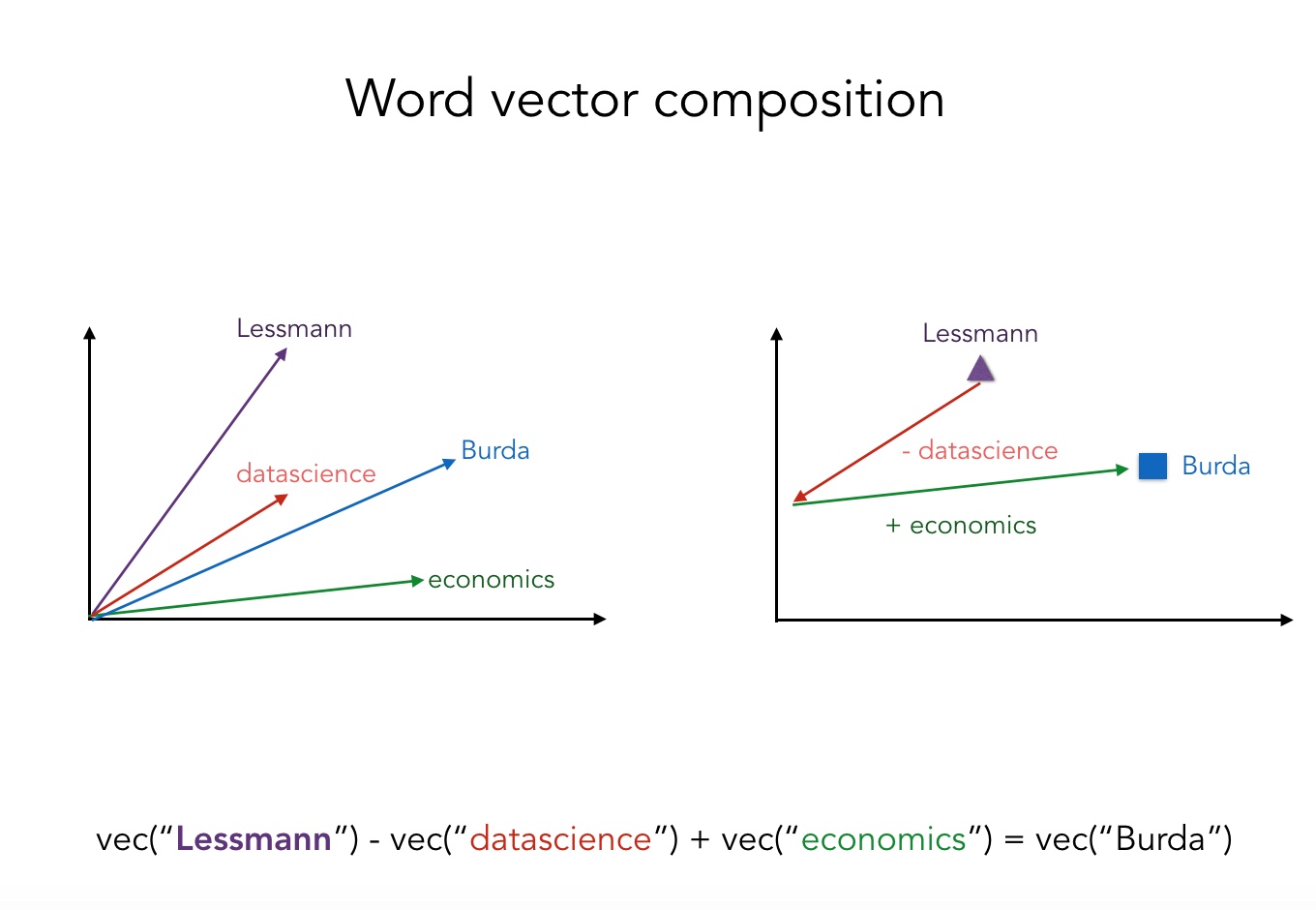
In reference to the famous king-queen example in the doc2vec literature, we test whether the models capture similar analogies. If we subtract ‘Frau’ from ‘Bundskanzlerin’ and add ‘Mann’ to it, we receive ‘martinschulz’ in the results. The similarity which the resulting vector shares with the word is rather weak:

similar words

Another nice feature is the fact that you can obtain the most similar word vectors for a word vector. We queried the model for several words that are shown next:

The end

If you made it till here, you have digested a lot of information, well done! We hope that our introduction to doc2vec gives you a better understanding of how PV-DBOW works. We would be happy, if you feel encouraged to apply doc2vec to some data on your own.