Image Analysis:
Introduction to deep learning for computer vision

Authors: Nargiz Bakhshaliyeva, Robert Kittel

In this blog, we present the practical use of deep learning in computer vision. You will see how Convolutional Neural Networks are being applied to process the visual data, generating some valuable knowledge. In particular, we focused on the object recognition task, aiming to classify what kind of an object (a dog or a cat) is presented within a particular image by using the notion of Transfer Learning.

But before diving that deep, let’s start from the very beginning.

A long time ago in a galaxy far, far away…human species decided to put all the burdens of straining their visual cortex on machines and artificial intelligence, and that’s basically how Computer Vision field was established.

Computer Vision: behind this fancy buzzword there is a notion of combining the implementation of visual-cognitive processes of the machines together with data-scientific approaches. Some notable applications of computer vision field include objects recognition and localization, human face detection, objects surveillance and tracking and many other problems.

What human eye and a computer sees differ drastically. For a machine, the visual information is being interpreted through pixelwise representation, with a pixel value representing a color or a brightness of it. Given specific bit storage representation, an image can be binary (1 bit) or grayscale (8 bit), with pixel values ranging from 0 (black) to 255 (white). A colored image is then comprised of 3 channels (red, green and blue) each within 8-bit structure. So, when dealing with visual information, computers input the data in form of pixel arrays in order to generate some valuable output information.

Feature Extraction

Recall the concepts of solving the traditional classification problems, where you deal with columns (vectors) of some variables representing the features required to predict the target class. But what is a feature in terms of image?

The features of images are depicted as small clusters of pixels of regions (also called keypoints), denoting edges, blobs, corners and so on. In order to detect these features, a variety of methods exists.

First, consider a rather traditional technique called SIFT (Scale-Invariant feature Transformations). A SIFT approach aims to generate features from images by creating feature vectors, which stay constant when an image is being geometrically transformed and/or rescaled. Let’s take a look at an example:

In the following coding snippets we use Python’s OpenCV API tool. Below, we created a shifted representation of the same image.

Now, how the SIFT features are computed? SIFT extracts the features as keypoints (interesting regions) along with descripting vectors. First, the keypoints are being searched for through filtering the scale-space of an image (varying sizes of windows for detection) and localized by selection of location candidates. Then, for each keypoint the orientation is being assigned in order to make them insensitive towards rotations. Next, keypoint descriptors in form of vectors of dimensions 128 x 1 are being created. Notice the circles on the images, those are exactly the keypoints:

Last but not least, in ordert to evaluate how precize and stable the keypoints are, we matched them on both images. As shown, most of the detected keypoints on both images are the same.

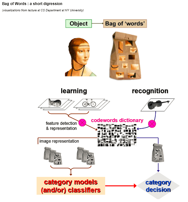
So, what is next? SIFT features can be fed to further algorithms to classify the objects on the images. One interesting approach is Bag-of-Visual-Words, where the features derived with SIFT are being clustered around the categories of the dictionary called „visual words“. Each part of the image is then mapped to a visual word being the center of a cluster. Having multiple visual words, the histogram of their occurencies is being computed which is then used in an arbitrary classification algorithm.

Another approach for feature extraction exhibits CNN’s ability to generate both low and high-level features. The extracted features are represented as activation maps created by the convolutional layer filters (with number of activation maps corresponding to the number of filters). The deeper the convolutions, the more sophisticated features are being generated. For instance, the first activation map may depict the basic keypoints such as circles or edges. The next activation map combines then multiple basic keypoints providing higher-level features. To demonstrate which features a deep network can learn, we built a simple CNN from scratch, training on the subsample of dogs&cats data. To keep it simple, we trained in 15 epochs (15 times passing the training data through the network), using 2040 training and 408 validation samples. As expected, the network was not able to learn quite well with final epoch validation accuracy of around 70%.

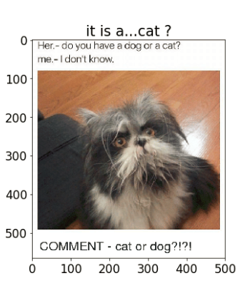
Quite surprisingly, this network was able to predict the class of a somewhat ambiguous image of a cat…

Okay, now back to the initial intention: what does the deep network learn? Here you can see which features (activation maps) the 3rd convolutional layer learns from a dog picture:

See the implementation below.

Image Augmentation

Before we start with actual classification experiments, we introduce the data augmentation technique. Data augmentation basically helps to overcome the scarcity of the training set by applying geometrical transformations to images (cropping, rotating, shifting etc). Thereby we synthetically increase the training samples processed by the network. In this manner, the network is able to better generalize on the test data, since with random image transformations fed in batches it almost never sees the same image again.

Affine transformations (rotation, shearing) involve geometric transformations with preserved parallel lines. To perform rotation, for instance, the center of an image is being defined. Given an angle theta for rotation, transformation matrix is computed and then multiplied with the original pixel coordinates to compute new coordinates.

Another example of geometric transformation is affine transformation, as implemented below.

Transfer Learning

CNN networks work in a way that in the bottom layers, only more general, low-level image features are identified, based on which the extraction of specialized high-level features (think e.g. of a whiskers of a cat) will be carried out on the top convolutional layers. Note that different image classification tasks (domains) share common feature space. Taking this commonness into consideration, one can state that features are distributed fairly uniform over domains of images. Therefore, a question arises: why one has to extract such features individually and over and over again, if they are general? This is where Transfer Learning concept comes into play.

Given the low-level features in networks being generic, the weights computed with CNN can be reused for other tasks. This is true if the base network that will be used for Transfer Learning is of the same structure as the base network where the learned feature weights come from. Thus, the base network trained with on the source domain is being adapted to the target domain by so-called fine-tuning, meaning the model is further learning the source domain. Moreover, state-of-the-art implementations impose an assumption of high correlation between source and target task domains.

Recalling our goal: classifying dogs and cat images.

To conduct the experiments, we incorporated basic VGG-16 architecture pre-trained on ImageNet without the classifier on top. Instead, we applied different optimized classifiers. For backpropagation, Stochastic Gradient Descent optimizer (SGD) together with a momentum of 0.9 and slow learning rate of 1e-4 was used, which ensures that the magnitude of updates stays small. A decision towards using SGD was mainly motivated by the previous findings emphasizing that the generalization ability on test data of adaptive optimization algorithms is worse than of SGD. Moreover, we use early stopping to stop training if the validation set accuracy doesn’t improve. Thereby we further regularize the model to prevent overfitting. The training dataset is relatively small with a sample size of 2000, the number of epochs defined at 50. To reduce the possibility of overfitting we add an “aggressive” dropout regularisation of 0.5 to the fully-connected layer. To improve training time we first use a ReLU activation function on the first fully-connected layer and then a sigmoid to create outputs, in order to obtain probabilistic outputs for the class of index 0 (cats).

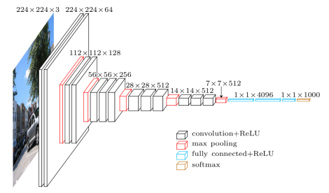(https://www.cs.toronto.edu/~frossard/post/vgg16/)

For further details check also Keras implementation API:
https://github.com/keras-team/keras/blob/master/keras/applications/vgg16.py

A function trainVGG16 expects as input the following parameters: boolean value of whether weights from pre-trained VGG16 model are used; a boolean value of whether dataset should be augmented or not; a number indicating at which layer depth to retrain. The latter is represented by a vector of layer numbers denoting the positions of the layers from top to bottom: [18, 14, 10, 6, 3, 0]. For instance, if the function is called with 18, no retraining will take place, meaning all layers are frozen. If the function is called with 3, all layers down to the 3rd will be retrained and so on. The parameterized call of the function results in 24 different models/combinations:

Once again: we start with the experiment when no layers are being retrained and then fine-tune the top layers, gradually going deeper down the architecture. To better visualize the results we use the notion of retraining in 6 blocks of layers in total: for instance, by saying that if block 3 is trained we imply that all top blocks above (Blocks 6, 5, 4 and 3) are being retrained as well.

The obtained results suggest that the more the retraining is drilled down, the more accurate the validation set performance was achieved, with best model having the setting of using pre-trained weights and data augmentation:

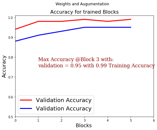
Additionally, in some experiments there is a tendency of increasing spread between train and validation accuracies with the increasing depth of the training. Moreover, the results indicate that it regardless of at which depth level the retraining starts, the combination of image augmentation and pre-trained weights always yields the best result when compared to other settings of having either image augmentation or incorporating weights or none of both. Another remarkable discovery is that pre-trained weights do not affect the validation accuracy to a degree augmentation does. Nevertheless, once again, it is somehow expected that the deeper the network is getting fine-tuned, the lower the impact of pre-trained weights since retraining deeper convolutions results in obtaining more task-specific filters and thus the pre-trained features are turning to be obsolete.
Subsequently, we applied our model to classify more distant domain. Having trained the network on the images of cats and dogs, we aimed to distinguish between the images of men and women. This time we compared this model to the usage of weights that were obtained by simply placing a classifier layer on top of the VGG16 network The best result of test accuracy of 99% was attained with a combination of pre-trained ImageNet weights and using no augmentation. Reconstruct the model structure to load the trained weights

And wrap the structure constructor with a function that builds the file names of all possible weight file, loads them and submit.

To sum up, we observed that it is worth to retrain (fine-tune) a network even when the pre-trained weights are available, which basically validates the concept of Transfer Learning. That is, in the setup we had, a maximum accuracy on validation set was gained after retraining the first four blocks (6,5,4,3), or, in other words, the top 14 layers. In short, relying on our results we suggest the following:

1. Utilizing the pre-trained weights if available
2. Taking advantage of data augmentation as long as the source and target domains are close
3. Retraining not just the top layer but deeper convolutional layers is rewarding. However, an even deeper training doesn’t improve accuracy much but can stimulate overfitting. Intuitively, the deepest convolutions retrieve the low-level features which are general to most of the visual data and hence do not differ much from the pre-trained features.