By Seminar Applied Predictive Modeling (SS19) | August 13, 2019
Revisiting Social Pressure and Voter Turnout: Causal Inference with Supervised Learning Methods
Julius Reimer & Toby Chelton
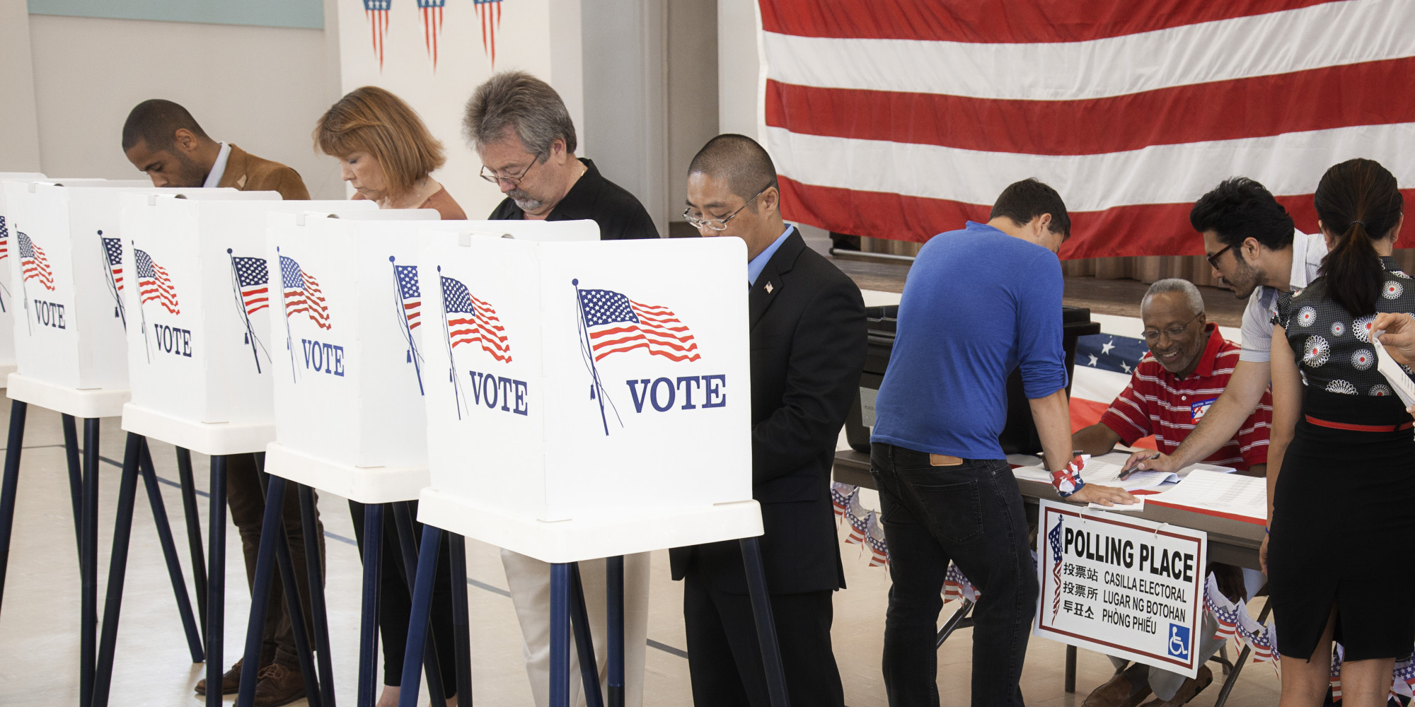
[Source: https://paulkiser.com/2016/02/04/five-fixes-for-our-primarycaucus-fiasco/]
Table of contents
2. Original Study and Our Objectives
1. Introduction
The issue of voter turnout has long been examined in both academic and media spheres. In fact, the interest dates back many years to papers such as Gosnell’s 1927 ‘Getting out the vote- an experiment in the stimulation of voting’. Many more academics followed this path like Powell (1986) ‘American Voter Turnout in comparative perspective’ - examining variance in turnout across developed democracies - and Geys (2007) ‘Explaining Voter Turnout: A review of aggregate-level research’ - an attempt to pin down some of the underlying factors behind turnout. These papers have thousands of academic citations according to Google Scholar. Meanwhile, stories such as the significance of youth voter turnout in European elections are widely reported and analysed in mainstream media. Perhaps there is an even greater interest than ever in this topic today, given the context of the rise in populism in Europe alongside threats to democracy from emerging technology.
In this post, we revisit the data from another widely-cited academic paper: Gerber et al.’s (2008) ‘Social Pressure and Voter Turnout: Evidence from a large-scale field Experiment’. By applying some of the latest methods in the emerging area of causal machine learning we build on the paper’s findings, specifically by investigating ‘heterogeneous treatment effects’. Our contribution is three-fold: first, we demonstrate the efficacy of causal machine learning models and compare their performance. Secondly, we uncover demographic trends in the original data that add further depth to the findings of Gerber et al., for example, the importance of age for the effectiveness of the treatment. The third key result in this post is how such methods can offer tangible benefits to practitioners in political science and consulting.
2. Original Study and Our Objectives
Gerber et al’s original study compared the effects of four different treatments on voter turnout in order to observe the significance of social pressure. The experiment was designed with a sample of 180,002 households in Michigan, prior to the August 2006 U.S. primary election.
The data was split into 5 groups. One control group including roughly 100,000 households and then 4 treatment groups of roughly 20,000. The households in a treatment group received one of four different mailers:
- Civic Duty - A simple call to “DO YOUR CIVIC DUTY - VOTE!”. This treatment serves as a baseline for the other three.
- Hawthorne - in the spirit of the famous Hawthorne experiment, this mailer informed the household that their voting behaviour was being studied: representing a mild form of social pressure.
- Self - this mailer takes the social pressure to the next level by showing the recent election participation of each individual in the household and promising to send a follow-up updated after the coming election.
- Neighbours - the fourth treatment was seemingly the strongest form of social pressure: the same as ‘Self’ but this time publishing the records not only of the household but also the closest neighbours on their street.
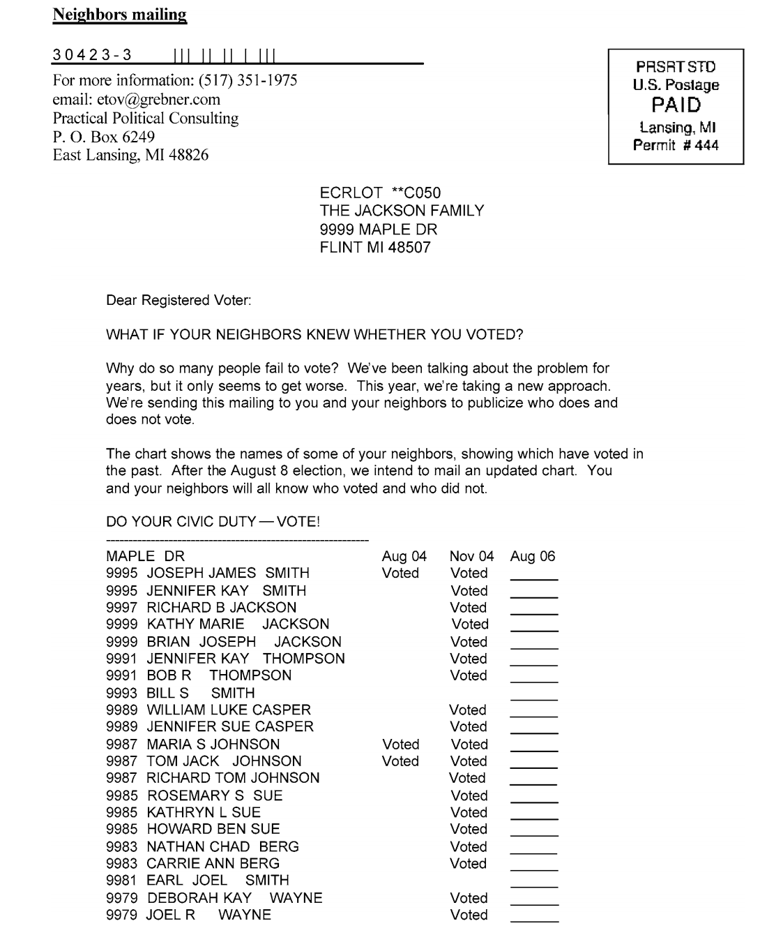
Fig. 1: The ‘Neighbours’ mailing (Gerber et al., 2008)
All four mailings can be found here.
Mailers were sent out in the days running up to the 2006 primary election. Due to the random assignment of treatment and control (which we explain later) and a large sample size, the treatment effect for each of the four mailers can be justified as equal to the difference in turnout rates between treatment groups and the control group. Their results were as follows and show the remarkably strong impact that social pressure was deemed to have had on turnout.
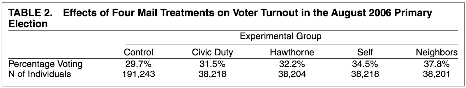
Tab. 1: Results from the original study (Gerber et al., 2008)
While Gerber et al. restricted their attention to average treatment effects, we want to build on their study by investigating heterogeneous treatment effects. In particular, we used supervised learning methods to estimate the conditional average treatment effect (CATE), which is defined as follows:
$$\tau(x)=\mathbb{E}[Y_i(1)-Y_i(0)|X_i=x].$$
In our application with a binary outcome variable $Y_i$, this is the difference in the probability of voting if treated and the probability if not, conditional on the covariates $X_i$, for individuals $i=1,…,N$. By finding out which groups of individuals were most reactive to the treatments, we can answer our key question: ‘Who should be targeted by these mailings?’. On the way, we will explore which characteristics of individuals are the most important for optimizing the campaign. The results then have the potential to be used by practitioners from political science or to consult on how such a campaign can be optimized in the future.
3. Data and Random Assignment
The authors provide the data set on two levels of aggregation: the household- and the individual-level. Throughout this post, we work with the more fine-grained individual-level data, containing information about more than 340,000 subjects. Although the number of observations emphasizes that Gerber et al. conducted a “large-scale” (p.33) experiment, the number of features for each observation is quite limited. An overview of them all is given in Table 2. Additionally to the outcome, indicating whether a person has voted in the 2006 primary elections, known characteristics are the sex, year of birth as well as the household size. It is further recorded whether a person has voted in the six general and primary elections between 2000 and 2004. We aimed to enrich the set of variables by computing averages by household, such as the average age. Moreover, we calculated the total number of previous elections, each individual has voted at. Given that information about six elections is available in the data, this feature would range between zero and six. However, the 2004 general election was excluded here and also from later analyses, since all subjects have voted at this election. In fact, participation at this election was one criterion, based on which the subjects have been pre-selected by the original authors. This brings us to the key question: how the treatment was assigned to subjects.
| Notation | Description |
| voted | Binary conversion indicator. It takes the value of one, if an individual has voted in the 2006 primary election and zero otherwise. |
| female | Binary variable that takes the value of one for females and zero for males. |
| age | The individual’s age in 2006. |
| hh_size | The size of the household an individual lives in. |
| p2000, p2002, p2004, g2000, g2002, g2004 | Six binary variables that take the value of one if an individual has voted in the primary (p) or general (g) election of the respective year and zero otherwise. The variable g2004 is excluded from all analyses here, because it is one for all individuals. |
| sum_votes | The number of previous elections, an individual has voted at, excluding the 2004 general election. |
| mean_[variable]_hh | The average value of [variable] by household. For example, mean_age_hh denotes the average age in an individual’s household. Household means are calculated for the following variables: age, female, p2000, p2002, p2004, g2000, g2002, and sum_votes. |
Tab. 2 Overview of variables
The treatment assignment is a crucial element of every experimental design with implications for which methods can be used for analysing the treatment effect. Here, the four treatments were randomly assigned, using the following procedure:
First, out of all households in the state of Michigan, several were excluded based on certain criteria. Probably the most important exclusion is that of households where all people were believed to be strong Democrats, with the reasoning that the analysed election was important mainly for Republicans. As indicated above, another criterion was that an individual must have voted in the 2004 general election, assuming “that those not voting in this very high-turnout election were likely to be ‘deadwood’—those who had moved, died, or registered under more than one name” (p.37). The households remaining after applying these two and some more criteria were sorted into an order required for mailing with the US Postal Service. After that, they were divided into groups of 18 households each and each group was sorted by a random number.
Although the authors state reasons for each step, their interventions raise the question whether the treatment can really be viewed as randomly assigned in the remaining data set. Therefore, we calculate variable means by treatment group, some of which are shown in Table 3. As shown, the averages differ only marginally across treatment groups, which supports the assumption of random assignment. Moreover, chi-squared tests were conducted, checking whether the variables are equally distributed in the different groups. All p-values were larger than 0.1, which is further evidence for the random assignment of treatments. The only exceptions, where the null hypothesis was not rejected, were the household size as well as the household mean variables, which we have created earlier. We presume that the reason is that the random assignment was done on a household-level, whereas the chi-squared tests - as all our analyses - were conducted on the individual-level.
| Treatment | female | age | g2000 | hh_size |
| Civic Duty | 0.5002 | 49.6590 | 0.8417 | 2.1891 |
| Control | 0.4989 | 49.8135 | 0.8434 | 2.1837 |
| Hawthorne | 0.4990 | 49.7048 | 0.8444 | 2.1801 |
| Neighbours | 0.5001 | 49.8529 | 0.8417 | 2.1878 |
| Self | 0.4996 | 49.7925 | 0.8404 | 2.1808 |
Tab. 3: Covariates’ mean values by treatment group
4. Modelling
Before turning to another crucial element of studying treatment effects, the models, the general estimation strategy should be explained. This is especially interesting, because instead of one, we analyse four different treatments here. The way we approach this, is to analyse each treatment separately. For each treatment, a different random sample of 38,000 control group observations is drawn. Since each treatment was given to approximately the same number of individuals, we have balanced data. The sampling of control observations is stratified on the outcome variable, i.e. the voting indicator for the 2006 primary election.
When having balanced data of approximately 76,000 cases for each treatment, this is split into a training and an estimation set with the ratio 70/30. The splitting is stratified on both the conversion indicator and the treatment indicator. The training set is then used for training the models, while the estimation set is “predicted” by the trained model, i.e. the treatment effect is estimated. This way, we avoid overfitting.
Having a total of four training and four estimation sets, we search for heterogeneous treatment effects using three different models. It is important to note that we used the same training and estimations sets for a certain treatment across all models, which ensures that the results are comparable. Our models are introduced in the following.
Logistic Regression (Logit)
The first model is a logistic regression with interaction term (Lo, 2002). A logit model - a binary outcome regressed on several covariates - is usually used for response modelling. The difference here is that in addition to the covariates, the treatment indicator is included as a regressor. Moreover, we include an interaction term with the treatment indicator for each covariate. The interaction effects allow for heterogeneity, because the marginal effect of the treatment now depends on the covariates’ values. To estimate heterogeneous treatment effects, the probability of conversion is computed with the treatment indicator set to one and a second time when it is set to zero. The difference between both probabilities is the estimated CATE. To allow for more complex relationships, quadratic terms have been included in the set of regressors.
As noted by Lo (2002), the approach of including interaction terms with the treatment indicator can also be used together with other supervised learning methods. A logistic regression, however, appeals for its simplicity and easy interpretation. A disadvantage is that we cannot include both the indicator variables for the previous elections and the total number of votes in these elections due to perfect multicollinearity. Since preliminary results and the findings of Künzel, Sekhon, Bickel, and Yu (2019) suggested that the total number of votes is a very important covariate, we decided to exclude the individual voting indicators.
Two-model
A simple approach that builds on standard learning algorithms to provide CATE estimates is often called the two-model approach. The data is separated into control and treatment groups and then for each group, a standard prediction model is trained, using all features apart from the control/treated indicator. Next, both models are applied to the estimation set giving both a prediction under control and a prediction after treatment for each observation. Finally, we take the difference between these two numbers as the estimated CATE for that observation. The validity of this calculation relies completely on the assumption of random assignment discussed earlier.
The advantages of this approach are both its simplicity as well as its flexibility, since it allows any non-causal learning model to be applied to each of the two groups. However, the approach is often used as a baseline model and is typically outperformed by other models. Radcliffe and Surry (2011, Section 5.1) suggest that the reason for its often lower performance is that since both models are trained independently, ‘nothing in the fitting process is (explicitly) attempting to fit the difference in behaviour between the two populations’.
The most important consideration in our implementation was that the two-model should be on a level playing field with the other approaches. For this reason, instead of training one model for the control group and then a model for each of the four treatments, we trained four pairs of models (therefore that included four separately trained models that all aim to predict voter turnout in the control group) using the same data sampling as we did for the other models. The base model that was used in every case was the XGBoost algorithm, tuned minimally using the MLR package for R.
Causal Forest
Similar to Breiman’s (2001) random forest for response modelling, which is an ensemble of many decision trees, a causal forest combines several causal trees into a treatment effect estimate. Causal trees were introduced by Athey and Imbens (2016) and developed further to causal forests by Wager and Athey (2018). The latest version of causal forests is described in Athey, Tibshirani, and Wager (2018). In fact, estimating heterogeneous treatment effects is only one special application of their so-called “Generalized Random Forest”. Together with this paper, the authors released the R package grf, which we use for implementing causal forests here.
Basically, there are two main characteristics that make causal forests different from the well-known random forests. First, their trees split the data as to “maximize the difference [i.e. heterogeneity] in treatment effect between the two child nodes” (Tibshirani, Athey & Wager, 2019). Secondly, they do not estimate the probability of response, but the treatment effect. It is worth to point out that - contrary to the logit and two-model approach - the causal forest estimates the CATE directly. The analyst does not need to take any differences or other transformations after estimation.
Moreover, we make use of an option proposed for causal forests, that is called “honesty”. This lets the causal forest split the data into two folds. Only the first fold is then used for growing a tree, i.e. determining the best split. After that, the second part of the data is used to calculate the estimations the tree will give. The clear disadvantage of making trees honest is that half of the data is wasted for both steps described above. However, honesty is one requirement that makes the forest’s estimations asymptotically normal (Wager & Athey, 2018). Together with variance estimates, this allows us to construct valid confidence intervals for the treatment effect (Athey, Tibshirani & Wager, 2018).
When implementing the causal forest, we use the package’s option to tune several parameters using cross-validation. For details, please refer to the package’s reference manual (Tibshirani, Athey & Wager, 2019). The only exception is the number of candidate variables for each split (mtry) for the ‘Neighbours’ treatment. In this case, the optimal value for mtry was found to be one, which we do not find sensible, as there would be only one candidate for each split. Therefore, we follow the rule of thumb for random forests, which suggests to take the square root of the number of variables, giving us a rounded mtry-value of four.
5. Results
From the modelling stage we arrived at 3 main results which will be explained in more detail:
- Our models predict significant heterogeneity in treatment effects
- Using causal models can add clear value to practitioners by suggesting which people to target
- Our results vary when comparing across models (as well as across treatments)
Heterogeneity and Variable Importance
Gerber et al’s (2008) study highlights the extraordinary impact that social pressure had on voter turnout in the Michigan primary. When you consider the long list of factors that might determine whether someone votes, and the fact that a single mailer to households of multiple people surely won’t even be seen by the entire treatment group, then the 8.1% turnout gain that they observe in the ‘Neighbours’ group cannot be understated. Nevertheless, what their study didn’t discuss is how this effect varied on a more granular basis. All of our models predicted quite a lot of variance within the estimation set.
Since all models predict an individual treatment effect for every individual in our prediction set, we can visualise the estimated heterogeneity by ordering the data by the predicted effect, grouping into quantiles (in our case deciles) and then for each decile calculating the average estimated treatment effect. In Figure 2 it is clear to see the variety in estimated treatment effect for the ‘Neighbours’ treatment.
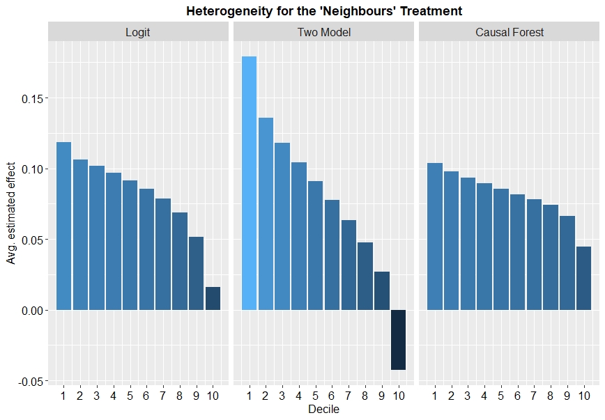
Fig. 2: Heterogeneity in treatment effect for the ‘Neighbours’ treatment
This comparison highlights a few points of interest:
-
All models predict that heterogeneous treatment effects exist in the data.
-
The extent of the predicted heterogeneity varies by model, with the two-model approach estimating much more variation than the causal forest and logit models.
-
It reminds us that for some individuals the treatment effect could even be negative.
We also see a similar trend for the 3 other treatments, but of course with (on average) lower values for the estimated effect.
Before going deeper into the analysis of how certain covariates relate to the treatment effect, we want to investigate which are the most important. The causal forest offers a method to estimate the importance of each variable. It is based on the number of splits, that are done on a variable in the top layers of the trees. Recall that the model aims to do splits that maximise the heterogeneity in treatment effect across the child nodes. Hence, the most important variables are those that have the largest impact on the CATE.
Figure 3 shows the causal forest’s variable importance for the ‘Neighbours’ treatment. The results do not differ a lot for the other treatments, i.e. Figure 3 is well-representative for all four treatments. The first observation we made is that the age, the total number of votes as well as their household averages are among the most important variables for all treatments. This means, the treatment effect for an individual differs depending on his/her age, the number of previous votes as well as certain household characteristics. Moreover, it was found that the individual voting indicators are rather unimportant across all four treatments. Interestingly, Figure 3 also shows that female is the least important variable, meaning that the treatment effect differs very little between males and females.
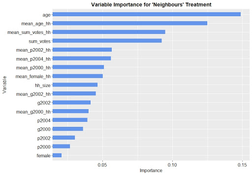
Fig. 3: Variable importance for the ‘Neighbours’ treatment
Who should be targeted?
Now that we found out that the treatment effect is different for people of different ages and with different participation in previous elections, we want to investigate how this relationship looks. This means, we want to find out, e.g whether old or young individuals have a larger treatment effect and should therefore be targeted with a mailing. To explore this kind of relationship, we use two different approaches. The first one is that we take the estimation set, we have split from the training set above, and estimate the treatment effects for these individuals. We can then investigate the relationship between the estimate and the individuals’ characteristics, e.g. by computing the average of the estimated effects for people with a certain age. The second approach is to use partial dependence plots, manipulating one variable in the training data and tracking how the model’s estimate changes, holding everything else constant. For both approaches, we show all plots together with a histogram of the analysed covariate. This allows to assess the uncertainty of the estimates, which is especially important for extreme covariate values. Furthermore, the estimations of the two-model approach proved to be very fluctuating, and giving some extreme values. We decided to limit the plots’ vertical axis, such that those extreme values are not always visible. Including these values would require a less granular scaled axis, thereby making more subtle trends almost invisible.
First, we focus on treatment effect heterogeneity depending on people’s age. Figure 4 depicts the estimated treatment effect averaged by age for the ‘Civic Duty’ treatment. As said above, the estimations of the two-model approach are highly fluctuating. Contrary to that, the differences in treatment effect estimated by the causal forest are smaller. What all models agree about, is that there seems to be a U-shaped relationship between the treatment effect and an individual’s age. This means the treatment effect is largest for people who are just older than 30 years, as well as for elderly people above 70 years. The curves indicate that the treatment effect becomes even larger for people above 80. However, as the histogram shows, there are few observations for very old people. Therefore, the estimates in these regions are rather not reliable.
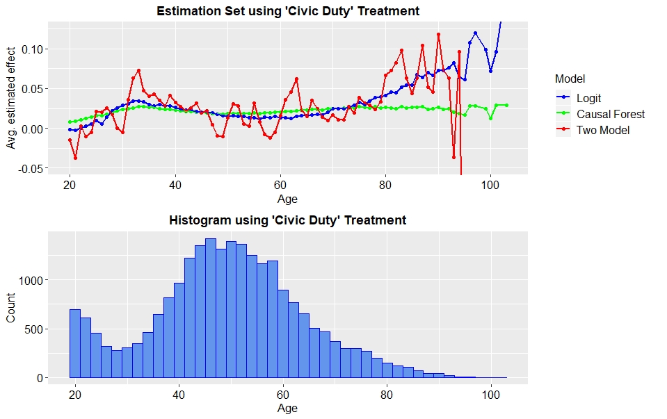
Fig. 4: Estimated treatment effects, averaged by age for ‘Civic Duty’ treatment
Next, the same analysis is done for the ‘Self’ treatment. The corresponding plots are shown in Figure 5. As shown, the story is a different one here. The logit and the causal forest both estimate a larger treatment effect for elder as compared to younger people. According to the logit, the treatment effect when targeting a 40 year old person is an increase in the probability of voting of approximately 4.1%. The treatment effect for a 70 year old person is 6.5% and hence considerably larger.
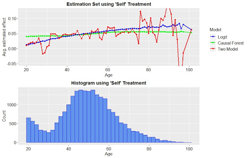
Fig. 5: Estimated treatment effects, averaged by age for ‘Self’ treatment
The comparison of results for the ‘Civic Duty’ and the ‘Self’ treatment shows that different groups of people may be better targeted with different mailings. While the call to the civic duty of voting appeals most to younger or elderly people, but not to those in between, the stronger form of social pressure exerted by the ‘Self’ treatment is more effective, the older the target is. The results for the remaining two treatments are briefly described in the following without showing the corresponding plots. For the ‘Neighbours’ treatment, the mailing seems to work best on people between 60 and 65 years. Moreover note, that the general level of treatment effect is larger for the ‘Neighbours’ treatment for many levels of age. The reason is that this treatment was the overall most effective, as shown by Gerber et al. Finally, for the ‘Hawthorne’ treatment, it is difficult to see any meaningful trend. The only conclusion that can be drawn is that this kind of mailing is less effective on individuals younger than 40.
Another important driver of heterogeneity for all four treatments was the total number of votes in previous elections. Figure 6 shows partial dependence plots for this covariate, when analysing the ‘Neighbours’ treatment. The treatment effect is comparatively small for individuals that have not voted in any of the primary or general elections between 2000 and 2004. It is larger for people having voted in some of the elections, and again smaller for those, having voted in all five elections. These results are very intuitive. Individuals that have never voted are probably hard to persuade to vote in the upcoming election. Opposed to that, individuals that have voted in all elections, are likely to participate in the next one even without treating them. The mailings have the largest effect on those who have voted in some elections, but not all. This group of people is maybe not fully confident in their decision to vote or not and therefore easy to influence. They should be targeted with the ‘Neighbours’ mailing.
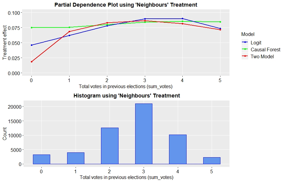
Fig. 6: Partial dependence plots for total number of votes and ‘Neighbours’ treatment
According to the logit model and the causal forest, results are similar for the other three treatments. The two-model approach shows different trends for the ‘Civic Duty’ and the ‘Self’. In particular, it suggests sending the first type of mailing to people having voted three or five times, whereas people having voted exactly two out of five times are most responsive to the latter.
The relationship between the household’s average age and the treatment effect is not entirely clear. While the logit model suggest that the overall relationship is negative for the ‘Civic Duty’, ‘Hawthorne’ and ‘Neighbours’ treatment, the two two-model approach does not indicate any clear trend. The only exception is the ‘Civic Duty’ treatment, where it agrees with the logit model’s findings. Contrary to that, the causal forest estimates a slightly positive relationship for the ‘Neighbours’ and ‘Self’ mailings. Interestingly, it also finds that households with an average age of approximately 35 are suitable targets for the ‘Hawthorne’ treatment.
Drawing an overall conclusion for the average number of votes in a household is even harder. If existing, trends differ by model and treatment. At least it can be stated that the ‘Neighbours’ treatment seems most effective for households with an average number of votes between two and four. This basically coincides with the findings for the individual-level number of votes.
It was discussed that - especially for the household characteristics - results differ significantly across models. They give different recommendations on what group of individuals to target. Practitioners might therefore want to follow the suggestions of the “best” model. The issue of which model is “best” is discussed in the following section on model evaluation.
Evaluating and comparing models
A predictive model is only as good as its ability to make accurate predictions on unseen data. Whilst this is fairly straightforward to compute in a typical prediction setting (albeit choices must be made about which metrics to use), the matter is complicated when considering treatment effects. The ‘fundamental problem of causal inference’ (Holland, 1986) is that for any individual we can only observe one of the two potential outcomes: the outcome under treatment or the outcome under control. It’s not possible to observe both and so we can never observe the ‘true’ treatment effect for any individual.
In light of this, one useful method we can use is the “Qini curve” and its coefficient. As outlined by Radcliffe (2007) this method requires us to rank our separate prediction dataset by the estimated individual treatment effect and then calculate the incremental gains at each segment (in our case deciles). The precise details of the calculation are not the main focus here but are outlined clearly in Radcliffe’s paper.
The higher the y-value of a point on a Qini curve, the better the model performs at that cutoff point. The Qini coefficient is then defined as the area between this curve and the straight line we would get for a random allocation of treatment (so, the higher the better). Figure 7 shows the Qini curves for our 3 models applied to the ‘Civic Duty’ treatment:
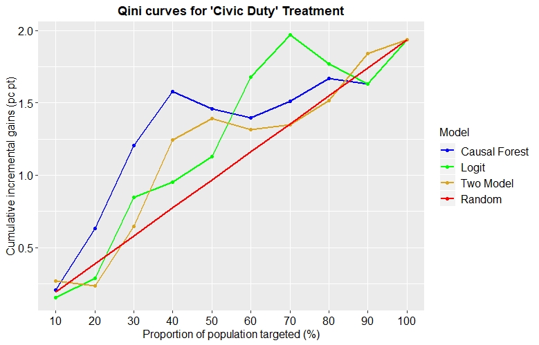
Fig. 7: Qini curves for each model applied to the ‘Civic Duty’ treatment
Suppose we were targeting 30% of the population. The Civic Duty treatment would be expected to induce roughly an incremental 0.6% of the total population to vote under random treatment assignment. If we instead assigned treatment to the most responsive 30% as predicted by the two model then the increment increases from 0.6% to around 0.7%. This reaches 0.8% and 1.2% for the logit and causal forest models respectively. (An interesting observation is that it is quite possible for the models to perform worse than random targeting at certain levels i.e. at 20% and 90%.)
From the image alone it’s not entirely clear which model is best. Whilst the causal forest dominates up to the 50% mark, the logit model then becomes better for targeting to 60%, 70% or 80% of the population. By calculating the Qini coefficient we are able to conclude that the random forest performed best for this treatment with a Qini score = 0.00257.
By replicating the same approach we see that the best performing model varies by treatment.

Fig. 8: Qini curves for each model applied to the ‘Neighbours’ treatment
And the following table summarises the results for all treatments and models:
| Qini Scores | |||
| Treatment | Logit | Two Model | Causal Forest |
| Neighbours | 0.00436 | 0.00466 | 0.00593 |
| Self | 0.00102 | 0.00163 | 0.00135 |
| Hawthorne | 0.00102 | 0.00668 | 0.00568 |
| Civic Duty | 0.00173 | 0.00105 | 0.00257 |
**Tab. 4: Qini scores by model and treatment**
This provides us with our overall conclusion about the competing performance of the models in this setting: Logit takes 3rd place, whilst Causal Forest and the 2-model approach are fairly even in 1st. Since Causal Forest performs best on the most effective treatment (by ATE), political campaigners would be advised to start with that combination in practice.
6. Conclusion
In this research, we have studied heterogeneous treatment effects with the example of voter mobilisation through four different mailings. In particular, we extended the findings of a widely-cited paper by Gerber et al. (2008) by investigating which groups of individuals the treatments were most effective on. We used three supervised models and found evidence that the treatment effect is indeed heterogeneous. The heterogeneity is mainly driven by an individual’s age and participation in previous elections as well as household characteristics. Investigating the relationship between treatment effect and covariates, it was observed that the results differed across treatments. This means, our recommendations on who should be targeted depends on the type of mailing. When using the highly effective ‘Neighbours’ treatment, individuals in their sixties, who have voted in the majority of but not all previous elections are most responsive.
We also found that results differed across models. Our evaluation of model performance suggested that the Logit model’s estimates are slightly less reliable than those given by the other two models. Perhaps the most important contribution we wanted to emphasise is that causal machine learning approaches can have a meaningful impact in a practical situation. The Qini curves clearly show that using models to target the most responsive individuals can be a significant improvement over random targeting. This means that a political campaign with a limited budget could make large improvements to their ROI by using these models.
Moreover, practitioners can not only target the individuals with the largest treatment effect, but also assess the uncertainty of this effect. Athey et al. (2018) showed that the causal forest’s estimations are asymptotically normally distributed. Together with the estimator for the treatment effect’s variance, it is possible to construct valid confidence intervals. To illustrate this point, Figure 9 depicts the estimated treatment effect together with the 95% confidence interval for six arbitrary individuals. We want to emphasize that this plot’s only purpose is illustrating the confidence intervals, even though it shows trends similar to the general results discussed above.
In Figure 9, the causal forest provides not only the information that the individual having voted in three previous elections has a treatment effect, that is considerably larger, but also assesses the uncertainty of the estimates. In this example, practitioners can be almost entirely sure that targeting the individual with three is more effective than targeting the person with two votes, since their confidence intervals do not overlap. Especially in the consulting industry, this theoretically proven information may convince potential clients.
Having emphasized the value of causal inference, the limitations in praxis should also be mentioned. Of course, there may be other considerations outside the scope of modelling such as whether or not the logistical costs of targeting specific individuals rather than certain zip codes outweigh the benefits. Moreover, the availability of suitable data is always an issue. Finally, it is important to note that there is not guarantee that the findings of this study would generalise to other conditions and elections. Especially since analysed individuals were mostly Republicans, it would be an interesting avenue for further research to investigate treatment effect heterogeneity in an election that is of interest also for Democrats. Nevertheless, the positive results from this research suggest that there will be many productive applications of causal machine learning models.
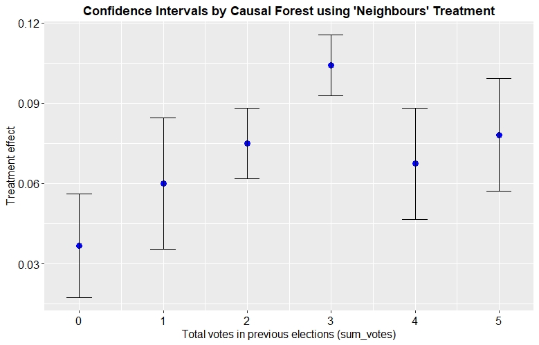
Fig. 9: Illustration of confidence intervals
7. References
Athey, S., & Imbens, G. W. 2016. Recursive partitioning for heterogeneous causal effects. Proceedings of the National Academy of Sciences, 113 (27), 7353-7360.
Athey, S., Tibshirani, J., & Wager, S. 2018. Generalized Random Forests. Available at: https://arxiv.org/abs/1610.01271.
Breiman, L. 2001. Random Forests. Machine Learning, 45 (1), 5-32.
Gerber A. S., Green, D. P., & Larimer, C. W. 2008. Social Pressure and Voter Turnout: Evidence from a Large-Scale Field Experiment. American Political Science Review, 102 (1), 33-48.
Gosnell, H. 1927. Getting out the vote–an experiment in the stimulation of voting. The Chicago University Press.
Holland, P. 1986. Statistics and Causal Inference. Journal of the American Statistical Association, 81 (396), 945–960_._
Künzel, S. R., Sekhon, J. S., Bickel, P. J., & Yu, B. 2019. Meta-learners for Estimating Heterogeneous Treatment Effects using Machine Learning. Available at: https://arxiv.org/abs/1706.03461.
Lo, V. S. Y. 2002. The True Lift Model - A Novel Data Mining Approach to Response Modeling in Database Marketing. ACM SIGKDD Explorations Newsletter, 4 (2), 78-86.
Radcliffe, N., & Surry, P. 2011. Real-World Uplift Modelling with significance-based uplift trees. White Paper TR-2011-1, Stochastic Solutions.
Tibshirani, J., Athey, S., & Wager, S. 2019. The GRF Algorithm. Available at: https://github.com/grf-labs/grf/blob/master/REFERENCE.md [last checked: 04/08/2019].
Wager, S., & Athey, S. 2018. Estimation and Inference of Heterogeneous Treatment Effects using Random Forests. Journal of the American Statistical Association, 113 (523), 1228-1242.