By Seminar Applied Predictive Modeling (SS19) | August 18, 2019
Applications of Causal Inference for Marketing: Estimating Treatment Effects for multiple Treatments
Authors: Jan Krol and Matthias Becher
Table of Contents
- Introduction
- Common Marketing Challenges
- Models
3.1 Decision Trees Rzepakowski & Jaroszewicz
3.1.1 Basic Rzepakowski & Jaroszewicz
3.1.2 Simple Splitting Criterion
3.2 Causal Tree and Causal Forest
3.3 Separate Model
- Evaluation Methods
4.1 Uplift Curves 4.2 Expected Outcome - Experimental Setup
- Results
- Outlook
- References
1. Introduction
Nowadays marketing practitioners face a multitude of challenges. In the first part of this blogpost we want to broadly look at some of the most common challenges and identify ways in which treatment effect analysis could be applied to tackle those challenges. In the second part we will focus more closely on one specific issue. Namely, estimating the effect of various treatments in order to select the best. To do that, we describe several models, which are applicable for modelling the uplift in the case of multiple possible treatment assignments. Later on we describe the difficulty of evaluating uplift models in contrast to classic machine learning models and describe two methods, which we use for our experimental evaluation. Afterwards, we describe our experimental setup and evaluate the performance of our implemented models, both in terms of their predictions and in terms of the duration it takes to train them. Finally, provide an outlook for further aspects that can be investigated.
2. Common Marketing Challenges
Some of the most commonly cited challenges we found were:
- Drive Traffic to the website
- Increase/Prove ROI of marketing campaigns
- Turn website visitors into buyers
- Reach people at the right time
- Target content to the right audience
- Select marketing channel/method
When?
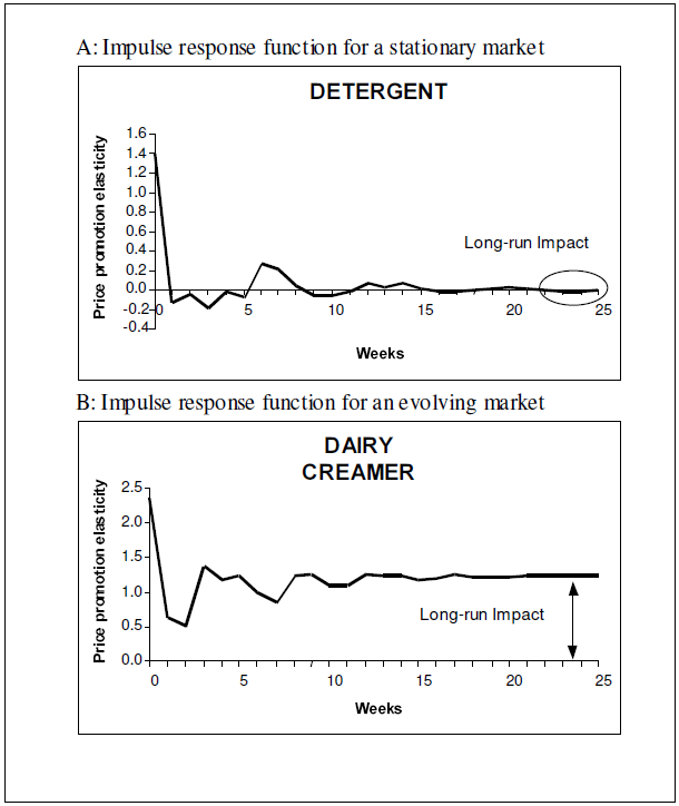
When it comes to selecting the time of a marketing activity there is not much research out there with regards to treatment effects. Most advice for marketing practitioners focuses on social media marketing and on the best publishing times for new posts. These guidelines mostly look at single performance measures like engagement to see at which times the performance measures are maximized. An example of this can be seen in the blog post “Best times to post on social media for 2019". Generally these approaches only attempt to maximize the average treatment effect. Social media usually works in a broadcasting style in which each post reaches all users. It is not possible to adjust the content or publishing time of a post for specific users or groups of users. In their paper Time Series Models in Marketing the authors look at the application of time series models for marketing. For example they use persistence modeling in order to estimate the long term effect of marketing activities. The image below shows the long term impact of an activity on the price promotion elasticity. For detergent there is an immediate effect, which levels off and reaches the original level after some time. For dairy creamer we also see some reduction over time but it remains stable at an elevated level.
Who?
The importance of this question varies greatly depending on the kind of marketing that is being done. Figure 2 shows various types of marketing from broad to narrow. The narrower, the more potential there is for the usage of treatment effects. For the broadest possible marketing activity (like the social media marketing mentioned before) the average treatment effect (ATE) is important but no selection can be made in terms of who we target. Narrower activities might allow us to select certain subgroups of our potential customers. Here we would be interested in the group average treatment effects (GATES) of those subgroups. Then we could determine which group to target based on those treatment effects.
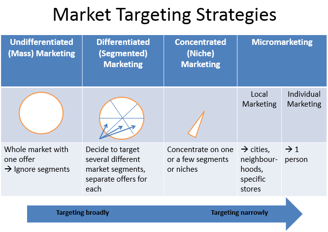
Our focus lies on the most narrow kind of marketing activities. This means activities like emails, coupons etc. which are specifically targeted towards the receiving person. Here we can decide on an individual basis whether we target a given potential customer and what treatment we use. This is in contrast to the broadest form, like social media posts, which reaches all followers and not just specific ones. Historically practitioners would target the people who they thought would be most likely to do a purchase. This approach is suboptimal since it is solely based on the overall purchase possibility and not the effect of the treatment. In general we can separate our customers in 4 groups (Figure 3).
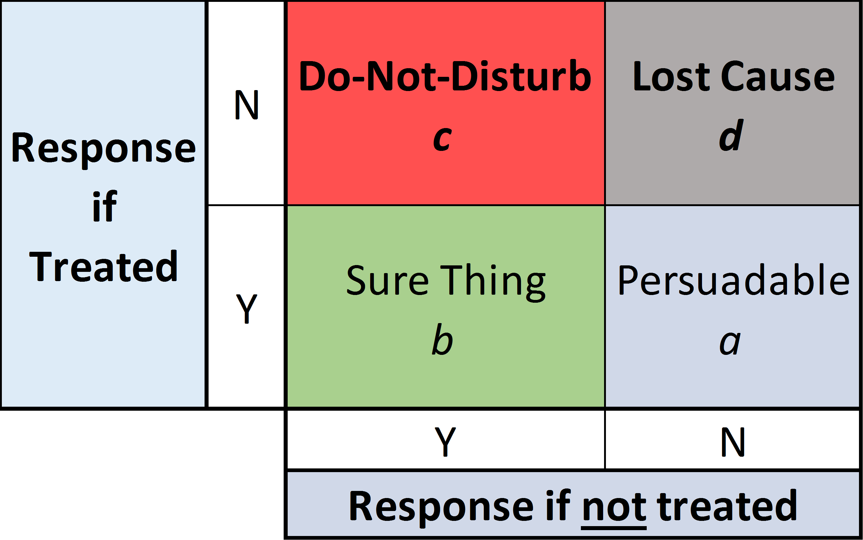
With the historical approach we will target mostly the ‘Sure Things’ and maybe the ‘Do-Not-Disturbs’. For those groups we at best get no return and at worst actually lose customers. Ideally, we want to target the ‘Persuadables’. This is commonly done by estimating the conditional average treatment effect (CATE) or uplift of the proposed marketing activity and then target the customers for whom the activity is estimated to have the highest effect. Several approaches have been proposed to estimate uplift. Gubela et. al (2019) give an overview in their paper Conversion uplift in E-commerce: A systematic benchmark of modeling strategies. In their evaluation they find that the two model uplift method and the interaction term method (ITM) performed best. The two model approach uses two separate models. The training set is split into two subsets. One subset contains all the treated observations and the other all control observations. For each training set one model is built to predict the outcome. To estimate the uplift of the treatment for a new person, we generate the predicted outcome with both models. One predicted outcome with treatment and one without. The difference between these two estimates is the expected uplift. The two model approach is very simple and works with virtually every possible base model (e.g. random forest, linear regression, svm, …). Since it is so simple it is often considered a good benchmark to test new approaches against. The interaction term method (ITM) was proposed by Lo in his 2002 paper The True Lift Model - A Novel Data Mining Approach to Response Modeling in Database Marketing. Unlike double machine learning, ITM only uses a single model. However, ITM also works with two predictions. One with treatment and one without. Both predictions are obtained from the same model which has been trained on both treatment and control data. Whether a treatment is given or not is indicated by a binary variable D. A new observation is evaluated twice. Once with D=1 (treatment given) and once with D=0. Again the difference between the two predictions is the estimated uplift.
What?
The last question we look at is “What marketing activity to choose?". There are many ways one could approach ones customers (e.g. coupons, newsletters, …). Finding the right method on an individual level is important, because different approaches might not only have different effects on potential customers but are also associated with different costs. For example it would be better to send a customer a newsletter which costs virtually nothing, rather then a coupon which would reduce profit, if the newsletter has a similar effect on purchase probability. Since there isn’t much research in this area and the selection of the proper marketing channel is crucial, we decided to lay the focus of our blog post on this issue.
3. Models
3.1 Decision Trees Rzepakowski & Jaroszewicz
3.1.1 Rzepakowski & Jaroszewicz Tree and Forest
In their paper Decision trees for uplift modeling with single and multiple treatments Rzepakowski and Jaroszewicz propose the usage of a decision tree for uplift modeling. The goal of their tree is to maximize the divergence of outcome distribution between the treatment(s) and control and between treatments. To that end they developed a splitting criterion used to evaluate the possible splits. For each possible split they calculate the associated gain. To put it simply the gain is the divergence of outcome distribution after the split (conditional divergence), minus the divergence prior to it (multiple divergence). The aim is to find the split, which maximizes the gain. The formula for calculating the gain is given below. $D$ represents a divergence function. In their paper they looked at KL-divergence, Euclidean distance and the chi-squared divergence. However, any other divergence measure could also be implemented. It is important to note here, that they only consider discrete outcome distributions in the paper. The gain: \begin{equation} D_{gain}(A) = D(P^{T_1}(Y),…,P^{T_k}(Y):P^C(Y)|A) - D(P^{T_1}(Y),…,P^{T_k}(Y):P^C(Y)) \end{equation}
Multiple Divergence: \begin{equation} {D(P^{T_1}(Y),…,P^{T_k}(Y):P^C(Y)|A) = \sum_a\frac{N(a)}{N}D(P^{T_1}(Y|a),…,P^{T_k}(Y|a):P^C(Y|a))} \end{equation}
With $a$ being one outcome of a given test and $N(a)$ the number of samples with outcome $a$ of that test. For example, let’s say we have $N = 1000$ people and we test for age below or above 25. Then $a_1$ would be $\leq25$ and $a_2$ would be $>25$. $N(a_1)$ are the number of people who are 25 or younger.
Conditional Divergence:
\begin{equation} D(P^{T_1}(Y),…,P^{T_k}(Y):P^{C}(Y))=\alpha\sum_{i=1}^{k}\lambda_iD(P^{T_i}(Y):P^{C}(Y))+(1-\alpha)\sum_{i=1}^k\sum_{j=1}^k\gamma_{ij}D(P^{T_i}(Y):P^{T_j}(Y)) \end{equation}
There are 3 parameters which can be set by the user to adjust the model. $\alpha$: This parameter determines how much the treatment-control and between treatment divergence are weighted. An $\alpha$ of 0.5 means both are valued equally.
$\lambda_{i}$: Allows to put an emphasis on certain treatments. For example, one might put more emphasis on cheaper treatments.
$\gamma_{ij}$: Allows to put individual weights on the divergence between certain treatments i and j.
In addition to the gain, they also added a normalization factor. In the equation below it is given for KL-divergence and entropy. It is supposed to prevent bias towards test with high number of outcomes. Additionally, it punishes uneven splits.
\begin{equation} I(A) =\alpha H(\frac{N^T}{N},\frac{N^C}{N})KL(P^T(A):P^C(A)) \end{equation} \begin{equation}
- (1 - \alpha)\sum_{i=1}^kH(\frac{N^{T_i}}{N^{T_i}+N^C},\frac{N^{C}}{N^{T_i}+N^C})KL(P^{T_i}(A):P^C(A)) \end{equation} \begin{equation} +\sum_{i=1}^k\frac{N^{T_i}}{N}H(P^{T_i}(A))+\frac{N^{C}}{N}H(P^{C}(A))+\frac{1}{2} \end{equation}
The first term measures the imbalance of the split between all the treatments combined and the control set. The second term measures the imbalance of the split for each treatment separately. The parameter $\alpha$ allows for setting the relative importance of those terms. The following two terms penalize attributes with large numbers of values by summing the test entropy over all the treatment and control datasets.
Lastly, pruning based on a validation set is also implemented. The pruning algorithm goes through the entire tree starting at the bottom. For each subtree the algorithm checks if the outcome divergence in the leafs is greater than in the root for the validation set. If yes, than the algorithm continues, if no the subtree is pruned and the root becomes a new leaf.
On the basis of this tree, we also implemented a function which allows to build a forest instead of just one tree. There are two main parameters which can be set when building a forest. The number of trees and the number of covariates considered in each tree. For each tree a random subset of the covariates with the specified number of covariates is used. Below is the process in pseudo code.
Forest building:

n_tree = 100 #The number of trees in the forest
n_features = 3 #The number of covariates used in each tree
forest = list()

Repeat #n_tree times:
  Randomly select #n_features of the covariates in the data and create a new subset of the data with those covariates
  Build a tree based on this subset
  Add the tree to the list of trees

For predictions:

predictions = list()

For each tree in forest:
  Make a prediction for the new sample and add it to the list

Return the average of all predictions
3.1.2 Simple Splitting Criterion
In addition to the tree proposed by Rzepakowski & Jaroszewicz we also implemented another splitting criterion as a benchmark. Unlike the previously discussed criterion, ours aims to maximize the difference in mean outcome between treatment and control and between different treatments. This also allows for continuous outcomes without any adjustments. There is no pruning implemented as we wanted to keep it as simple as possible. For that reason we also only compare the difference in outcome of the left side of a new split to the root in order to get the gain of a give split. Despite our effort to keep this criterion simple, we implemented a normalization factor which is used to guarantee that we have at least one observation of each treatment and control in every leaf. In addition, it also punishes uneven splits. Here is the formula used to evaluate the possible splits. The “$S = l$” indicates, that we are only looking at the left side of the split. $n_{il}$ and $n_{ir}$ are the number of samples with treatment i in the left and right leaf respectively. As one can see if either becomes 0 the whole equation is 0. \begin{equation} \sum_{i=1}^{I}\sum_{j=1}^{I}[Mean(Y|T_i=1,S=l)-Mean(Y|T_j=1,S=l)]^2*\prod_{i=1}^I\frac{n_{il}}{n}*\frac{n_{ir}}{n} \end{equation} Pseudo code for the simple tree:
Build_tree(data){
  For each split:
    Split the data
    Calculate and save the gain (equation above)
  If max(gains) > 0{
    Select split with highest gain
    Split the data according to the split in data_left and data_right
    Left leaf = Build_tree(data_left)
    Right leaf = Build_tree(data_right)
  }
  Else{
    Calculate mean outcomes for all treatments and control (these outcomes serve as predictions)
    Return(outcomes)
  }
}
3.2 Causal Tree and Causal Forest
The causal tree, introduced by Susan Athey et. al in their paper An Introduction to Recursive Partitioning for Heterogeneous Causal Effect Estimation Using causalTree package is a tree based classifier which directly estimates the treatment effect. It is based on the rpart package and implements many ideas in the CART (Classification and Regression Trees). By default it only supports single treatment. Therefore, we train one tree for each of the multiple treatments and then compare the predicted uplifts. They also implemented a function which allows the user to build forests based on the causal tree. These forests are in the form of a list of rpart objects.
3.3 Separate Model Approach
The two model approach for uplift models can also be extended for the case of multiple treatments.
We adapt the naming convention from Zhao et al.(2017) and depict it as the separate model approach (SMA).
With multiple treatments, for each treatment and the control group a separate model is trained.
The predicted uplift for an individual $x$, for every treatment $T$ is than calculated as:
\begin{equation} \text{uplift}^T(x) = P(Y^T | X) - P(Y^C | X) \end{equation}
Where $X$ depicts the covariates for the subject $x$, which are used by the base learners to predict the outcome $Y$.
For the SMA any prediction model can be used as the base learner, to model the response of a group.
This makes the performance of the SMA highly dependent from the choice and model specific tuning of the base learners.
The training objective of the base learners is to model the response of the underlying treatment or control group.
The effect of the treatment itself is estimated later, which makes the SMA an indirect uplift modelling approach.
Therefore, in the literature it is often advised to use a direct approach, which aims to model the actual difference between the treatment and control classes (Zhao et al. 2017).
4 Evaluation Methods
In contrast to a usual prediction task, it is not possible to observe the actual outcome of a subject for all possible treatment assignments (including no treatment assignment).
Therefore, standard machine learning measures are not applicable to evaluate the performance of an uplift model.
In order to approximate the actual gains of using the predictions from an uplift model, some assumptions need to be made.
We describe two approaches from the literature which can be used to compare the performance of different uplift models.
4.1 Uplift and Qini Curves
Both uplift curves and qini curves build upon the idea of cumulative gain charts.
Those require all targets to be ranked in descending order by their score.
For the single treatment case the score represents the uplift when assigning the treatment to the subject.
In the case of multiple treatments the uplift model predicts the uplift for each treatment. The score then corresponds to the maximal uplift of all possible treatment assignments.
In case the uplift for all treatments is negative, the score can also be negative. This corresponds to the behavior of the ‘Do-Not-Disturbs’ group.
Given the ranked outcomes for each treatment and the control group, a cumulative lift curve can be drawn.
The x axis represents the number of treated subjects and the y axis the cumulative outcome.
The uplift curve represents the lift curve for a treatment, subtracted by the lift curve of the control group.
The main assumption of this approach is that similarly scored groups inhibit similar features and are therefore comparable.
However, Rzepakowski et al. (2012) mention that this property is not necessarily satisfied, but currently no better alternatives exist.
As the treatments and control groups in the testing dataset can have different sizes, their outcomes need to be scaled in order to represent a meaningful subtraction of the treatment and control outcomes.
Here the difference between the qini and uplift curves becomes apparent.
The qini curve as described by Radcliffe et al. (2007) scales the outcomes to the sample sizes of the treatment group.
\begin{equation} f(t) = Y_t^T - \frac{Y_t^C N_t^T}{N_t^C} \end{equation}
With $t$ as the quantile for the amount of the treated population, $T$ as the treatment assigned and $C$ as the Control group. $N_t^T$ and $N_t^C$ depict the number of subjects in the according treatment and control group, within the top quantile. $Y_t^T$ and $Y_t^C$ stand for the total response in the treated group within the top quantile.
The uplift curve, as described in Gutierrez et al. (2017), uses the sample mean of each group and scales it to the full sample size.
\begin{equation} g(t) = \Bigg( \frac{Y_t^T }{N_t^T} - \frac{Y_t^C }{N_t^C} \Bigg) \big( N_t^T + N_t^C \big) \end{equation}
In the case of multiple possible treatment assignments, naturally for each treatment a separate uplift curve can be drawn.
In order to derive a combined curve for all treatments, it is possible to combine all treated subjects as one group and compare their outcomes per ranked quantile to the control group.
Additionally, the uplift per subject can then be upscaled for the whole testing group $N_t$.
\begin{equation} g(t) = \Bigg( \frac{Y_t^{T^\prime} }{N_t^{T^\prime}} - \frac{Y_t^C }{N_t^C} \Bigg) N_t \end{equation}
We denote the combined group of all possible treatments with $T^\prime$. This group is than scored and ranked as a whole by their maximal uplift value.
As the qini curves are scaling towards the treatment sample size, a combination of multiple treatment groups with different sizes becomes more cumbersome.
Therefore, we see the uplift curves more applicable for multiple treatments and discard the qini curves in our experimental evaluations.
4.2 Expected Outcome
Another evaluation method for uplift models with multiple treatments is the expected outcome metric propose by Zhao et al. (2017). It estimates the expected outcome, given that each subject is assigned the treatment with the highest outcome, predicted by the uplift model (including choosing no treatment).
The authors define a random variable $Z$ as
\begin{equation} Z = \sum_{t=0}^{K} \frac{1}{p_t} Y I [h(X)=t] I [ T=t ] \end{equation}
where $I$ depicts the indicator function, $p_t$ the probability that the assigned and predicted treatments have been matched and $h(X)$ the predicted treatment by the uplift model.
In case the treatment predicted by the uplift model is equal to the actual assigned treatment to the subject during the experiment, the weighted outcome of this subject is summed.
In other words, the subjects where the predicted and assigned treatments match, form the group of representatives for those with this treatment assigned.
As the number of matched subjects can vary, their group outcomes are then weighted.
The expected value of $Z$ is than equal to the expected outcome, given that each subject is assigned the best predicted treatment, as shown by the authors.
Furthermore, the sample average $\bar{z}$ represents an unbiased estimate of $E[Z]$.
\begin{equation} E[Z] = E[Y|T=h(X)] \end{equation}
\begin{equation} \bar{z}=\frac{1}{N} \sum_{i=1}^{N}z^{(i)} \end{equation}
The expected response can also be used to draw uplift curves. In Zhao et al. (2017) those curves are named modified uplift curves.
Once again the subjects are ranked by their score (expected uplift). Now for the top t-percent the optimal treatment is assigned and the remaining subject are assigned to the control group.
Now the expected value for treating t-percent of the subjects are given as $\bar{z}$.
In contrast to the qini and uplift curves, the modified uplift curve is not cumulative, as the outcomes of the not treated subjects are also taken into account.
Also the expected outcome is defined per customer and therefore independent from the size of the testing data.
This can make it easier to draw decision in a business setting, as the expected per customer returns can be easily scaled to the planned marketing campaign sizes.
5. Experimental Setup
Data Set
We use the E-Mail campaign dataset from Kevin Hillstrom’s MineThatData for our evaluation.
This dataset represents a randomized E-Mail marketing campaign of an online vendor with two treatments (Mens E-Mail, Womens E-Mail) and a control group.
The dataset consists of 64,000 observations, 3 target variables and 8 feature variables.
The measured outcome variables are whether the customer visited the website or if he actually converted, which are both binary.
Furthermore, also the actual spend of the customers is measure, which represents a continuous outcome.
As shown in Table 1 the total response rates for all outcome variables are quite low.
When looking at the two E-Mail campaigns in Table 2 both treatments have a total positive effect on all target variables.
As the dataset is already preprocessed we did not had to do any manipulations to the data.
| AVG Response | |
|---|---|
| visit | 14.68% |
| conversion | 0.90% |
| spend | $1.05 |
| visit | conversion | spend | |
|---|---|---|---|
| Mens E-Mail | 7.66% | 0.68% | $0.77 |
| Womens E-Mail | 4.52% | 0.31% | $0.42 |
Implementation
Using the E-Mail campaign dataset, we have evaluated our implementations of the described models.
We have implemented the trees from Rzepakowski et al. (2012) with multiple possible divergence measures and the described splitting criteria in R.
We have also built a forest model with those trees as the subtrees. Unfortunately it did not result in a significant improvement.
Therefore, we did not include them into our evaluation.
For the causal forest we use the available implementation from Athey et al. (2016).
We build the causal forest using 200 subtrees and a mtry parameter of 2.
For the SMA we have evaluated several possible base learners and chose a tuned random forest as it performed best in our experiments.
We have fitted and evaluated all models using 5 fold cross validation and set a seed beforehand, in order to avoid inconsistencies in the outcomes due to different evaluation data splits.
The full implementation of our models and evaluation metrics is shared on GitHub.
6. Results
Predictive Results
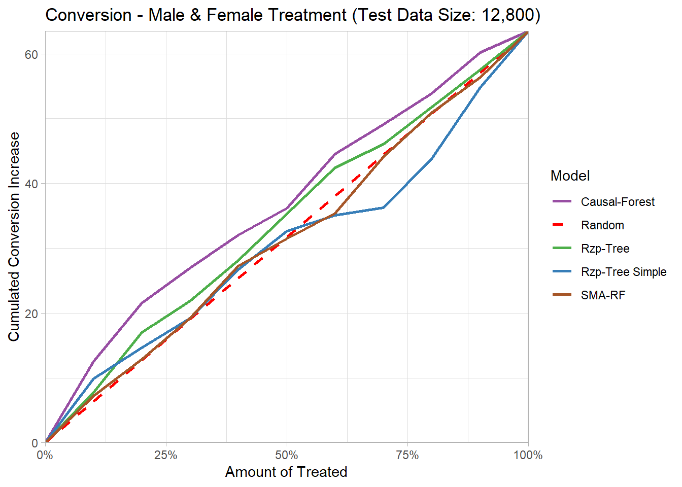
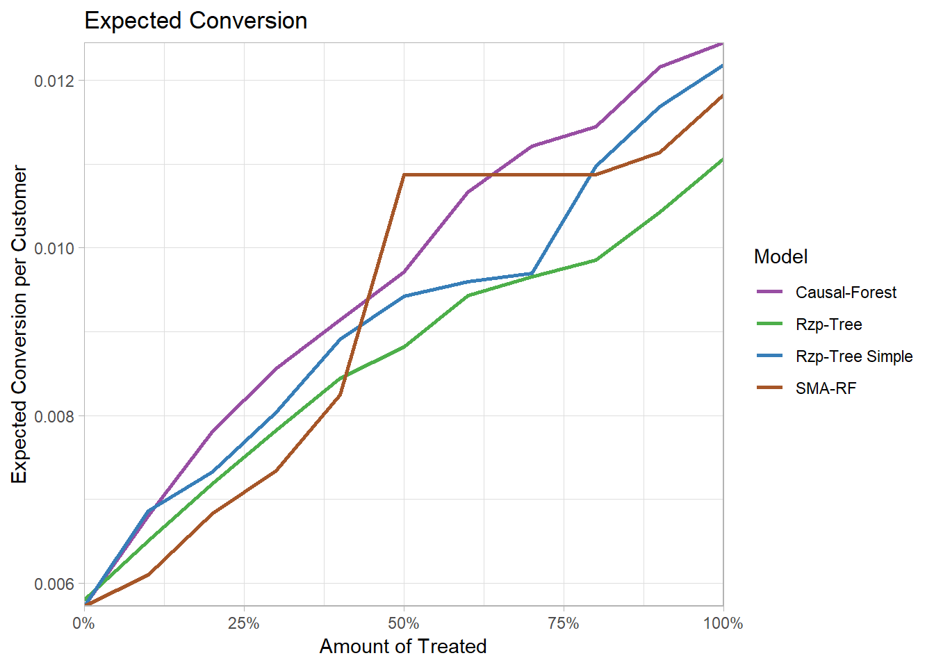
When looking at the uplift curves for the conversion, we can see that all models are very close to the random assignment.
Also as the cumulative curves are constantly rising, the E-Mail campaign seems not include a large number of ‘Do-Not-Disturbs’.
The same applies for the expected conversion per customer.
Due to no early rising of the curves and the overall positive treatment effect of the treatments, from a marketing perspective it would be best to target as many customers as possible, within the marketing budget.
The flat plateau for the SMA model in the expected coversion, is due to the fact, that the RF model has less than 10 leaf nodes.
Therefore, when calculating the deciles for the ranked test subjects some decile segments did were the same.
The causal forest slightly outperforms the remaining models, while still being close to a random treatment assignment.
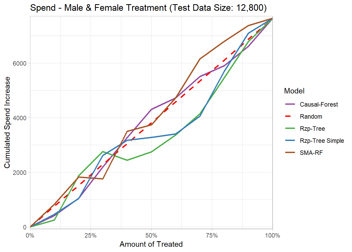
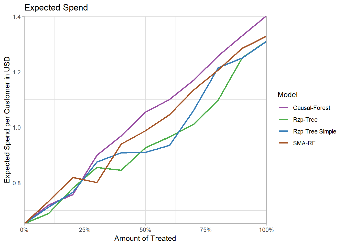
Also in case of the continous spend target variable, the results are close to a random assignment.
The causal forest once again slightly outperforms the other models, while the trees from Rzepakowski et al. (2012) perform even worse than random.
We assume that the better performance of the causal forest might be due to the fact that it consists of 200 subtrees.
However, it is still interesting that it outperforms the trees from Rzepakowski et al. (2012), as the causal forest consists of separate causal forest for each treatment and cannot consider both treatments while training.
Training Duration
Even though predictive performance is the focus of this evaluation we also wanted to look at how well our approaches scaled in terms of training duration. The are 3 factors we looked at which will influence performance: number of observations, number of covariates and number of treatments. The causal forest consists of 100 trees and randomly selects 3 covariates for each tree. The forest on the basis of the Rzp-tree is not in the comparison. This is due to the fact, that its training duration was up to 10 times the one of the base tree. Therefore it was omitted for readability of the graphs. It is important to note that parallelization is not implemented yet, which could reduce the training duration significantly. The figures below show a comparison of our models.
3 Covariates:
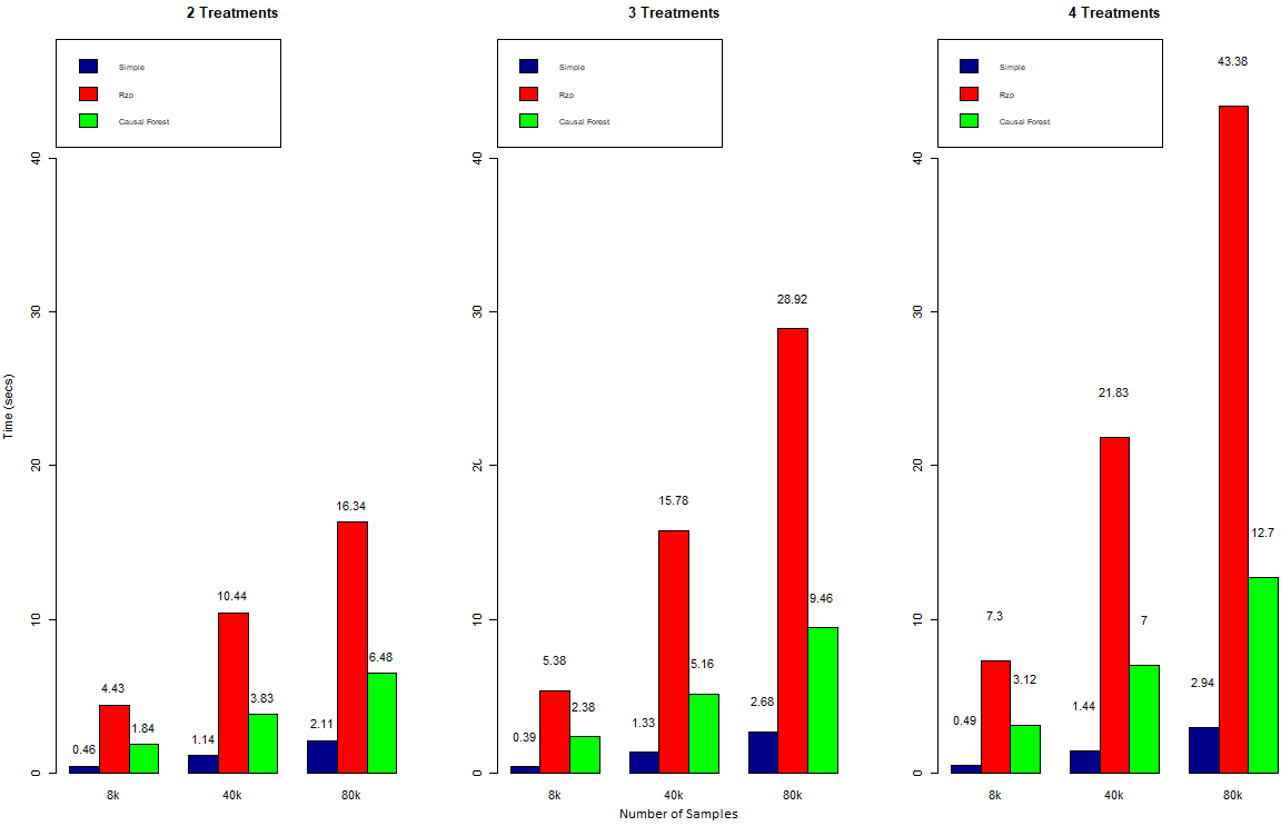 As one would expect, training duration increases with an increasing number of observations and possible treatments. The increase is roughly linear or a little less. Overall, the Rzp-tree has by far the highest training duration. This could either be a result of the design or due to poor optimization in the implementation.
4 Covariates:
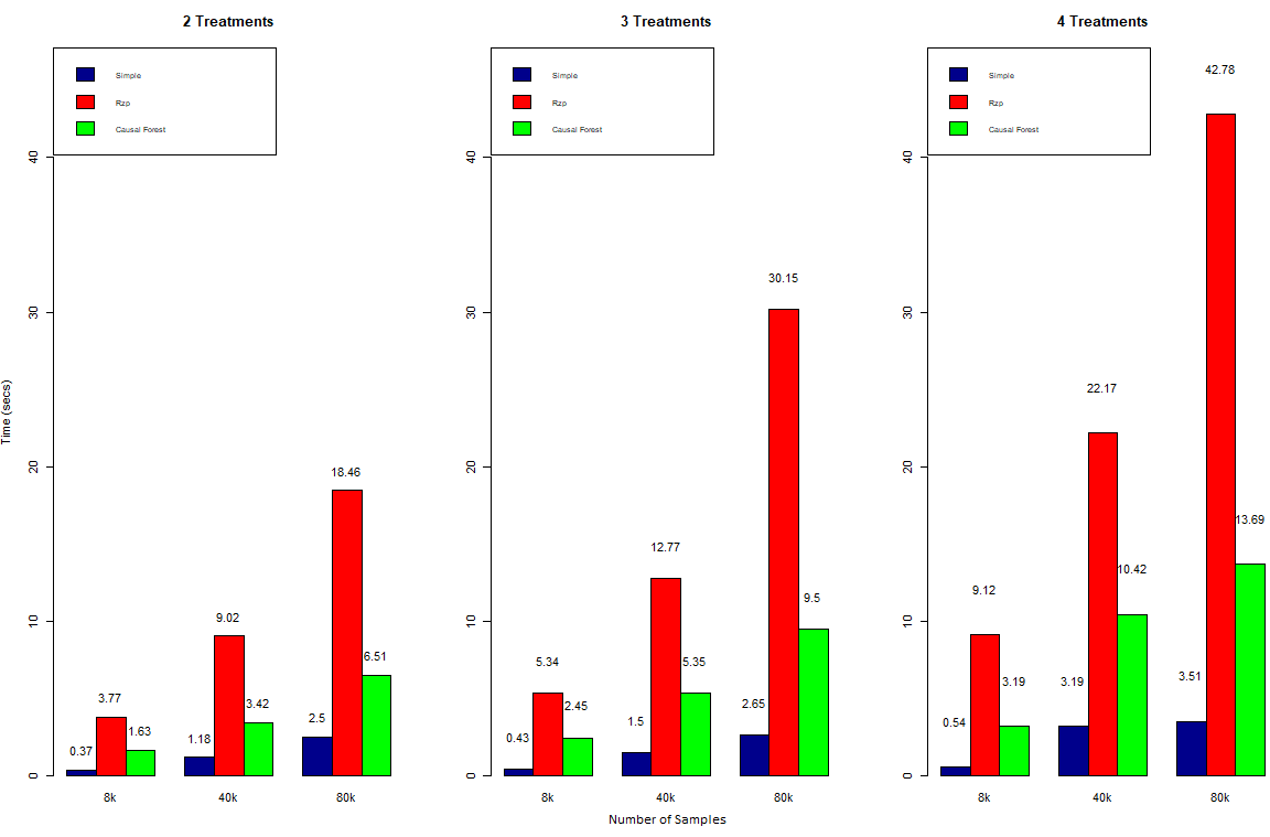 The added covariate was random binary, which means it has no predictive power. For the trees this additional covariate leads to one more potential split which has to be evaluated. As we can see this has virtually no effect on training duration.
5 Covariates:
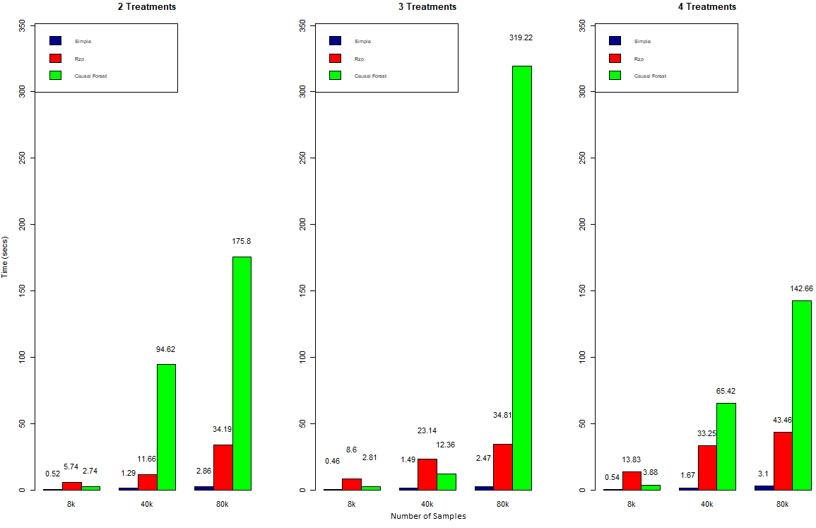 The second covariate which was added was a continuous variable which can take integer values from 0 to 100. It too was randomly assigned. Here we see hardly any effect on the simple tree and some effect on the Rzp-tree. By far the biggest effect is observed for the causal tree. Especially for higher numbers of observations the training duration increases significantly. It is interesting to see that the highest training duration is for 3 treatments instead of 4. This is likely due to ‘bad luck’ when selecting the covariates for each tree, often selecting the continuous rather than binary covariate.
7. Outlook
Unfortunately, our evaluation using the E-Mail campaign dataset provided mixed results, so that it cannot be clearly said which model would be most applicable for a marketing campaign.
The causal forest, as an ensemble model, did perform slighly better than the remaining models. Therefore, it would be interesting to compare a forest model from the proposed trees, which considers all treatments while training.
In terms of runtime, the key take away is that causal tree seems to struggle with continuous variables. For data with many continuous variables one should consider other models.
Overall, the rather poor results show, that there is still much room for improvement and further research on this topic.
8. References
- Athey, S. and Imbens, G., 2016. Recursive partitioning for heterogeneous causal effects. Proceedings of the National Academy of Sciences, 113(27), pp.7353-7360.
- Devriendt, F., Moldovan, D. and Verbeke, W., 2018. A literature survey and experimental evaluation of the state-of-the-art in uplift modeling: A stepping stone toward the development of prescriptive analytics. Big data, 6(1), pp.13-41.
- Gubela, R., Bequé, A., Lessmann, S. and Gebert, F., 2019. Conversion uplift in e-commerce: A systematic benchmark of modeling strategies. International Journal of Information Technology & Decision Making (IJITDM), 18(03), pp.747-791.
- Gutierrez, P. and Gérardy, J.Y., 2017, July. Causal inference and uplift modelling: A review of the literature. In International Conference on Predictive Applications and APIs (pp. 1-13).
- Lai, Y.T., Wang, K., Ling, D., Shi, H. and Zhang, J., 2006, December. Direct marketing when there are voluntary buyers. In Sixth International Conference on Data Mining (ICDM’06) (pp. 922-927). IEEE.
- Lo, V.S. and Pachamanova, D.A., 2015. From predictive uplift modeling to prescriptive uplift analytics: A practical approach to treatment optimization while accounting for estimation risk. Journal of Marketing Analytics, 3(2), pp.79-95.
- Radcliffe, N.J., 2007. Using control groups to target on predicted lift: Building and assessing uplift models. Direct Marketing Analytics Journal, 1, p.1421.
- Rzepakowski, P. and Jaroszewicz, S., 2012. Decision trees for uplift modeling with single and multiple treatments. Knowledge and Information Systems, 32(2), pp.303-327.
- Zhao, Y., Fang, X. and Simchi-Levi, D., 2017, June. Uplift modeling with multiple treatments and general response types. In Proceedings of the 2017 SIAM International Conference on Data Mining (pp. 588-596). Society for Industrial and Applied Mathematics.
- Dekimpe, Marnik & Franses, Ph.H.B.F. & Hanssens, Dominique & Naik, Prasad. (2006). Time-Series Models in Marketing.
- Lo, Victor. (2002). The True Lift Model - A Novel Data Mining Approach to Response Modeling in Database Marketing.. SIGKDD Explorations. 4. 78-86.

