By Seminar Applied Predictive Modeling (SS19) | August 15, 2019
Microfinance Policies
Impact of Microfinance on The Social Well-being
Authors: Edanur Kahvecioglu and Yu-Tang Wu
Abstract
Is microcredit a miracle or just a hype? While more and more researches were conducted to study microcredits, people started to question the effectiveness of microcredit program. This project explores the heterogeneity of treatment effect on microcredit to households’ well-being. Causuall Random Forest and Two-model approach are used to analyze treatment effects on the household level and identify the important variables that separate households with higher treatment effect. The results show evidence of heterogeneity of the conditional treatment effect on certain aspects of well-being. In addition, policy suggestions are proposed to attempt to increase the performance of microfinance program.
Table of Contents:
- Motivation
- Introduction
- Dataset
- Methods
- Results
- Model Comparison
- Interpretation And Policy Suggestions
- Conclusions
- References
Motivation
Microfinance is a type of credit provided to unemployed or low-income individuals or groups who are deprived of having access to conventional financial services. Although it is not a new concept in human history, as a first organization, Grameen Bank was established in 1976 by Muhammad Yunus in Bangladesh. It provided small loans to the poor without requiring collateral. The idea was very promising and it even brought Yunus a Nobel Prize. However, since the 2010 Indian Microfinance crisis, its effectiveness is in doubt and being discussed (Mader 2013). According to Banerjee et al. (2015) though, microcredit institutions have been effective for business and social well-being to a certain extent. For the assessment of the impact of microcredit institutions in the treated area, they used OLS regressions with area-level control variables and the indicator for living in a treated area.
$$y_{ia}=\alpha+\beta*Treat _{ia}+X _{\alpha} ‘\gamma +\epsilon _{ia}$$
However, usage of OLS arose two backlashes which this paper tries to challenge.
First, it assumes if there is a statistically significant on an indicator, which happened after the experiment being carried out, then the change must be a result of the treatment. However, it fails to distinguish people who would have increased or decreased their well-being regardless of the treatment, in this case, the introduction of microcredit institutions.
Second, it calculates average treatment effects in the area which is the difference in average outcomes between areas assigned to the treatment and areas assigned to the control. By calculating the average effect, it fails to capture the subgroup in the area which caused the major difference among the ones who may not have been affected by the treatment. Heterogeneous treatment effect, on the other hand, could have been useful to differ the subgroups which are affected most from the least.
In this paper, the dataset from (Banerjee et. al. 2015) has been used in several uplift models to capture the heterogeneous treatment effect of easy access to microcredit in the treated areas. By doing so, it is aimed to find the most affected subgroups from the treatment and to come up with policy suggestions for the microfinance institutions accordingly.
Introduction
Since the dataset from (Banerjee et. al. 2015) paper is used, it was important to understand how the data is collected and the experiment is pursued.
The paper (Banerjee et al. 2015) presents the results from the randomized evaluation of a group-lending microcredit program in Hyderabad, India. Microcredit has been lent to groups of 6 to 10 women by a microfinance institution, Spandana. According to the baseline survey conducted in 2005, 104 neighborhoods with no pre-existing microfinance was selected. They were paired up and one of each pair was randomly assigned to the treatment group. Spandana then progressively began operating in the 52 treatment areas between 2006 and 2007. As an important point to highlight, the treatment was not a credit take-up but an easy access to microcredit.
This first endline survey was conducted at least 12 months after Spandana began operating within a given area, and generally 15 to 18 months after, which corresponds to the dates 2007 and 2008. Two years later, in 2009–2010, a second endline survey, following up on the same households, was undertaken. In the surveys, the questions related to the households’ business, consumption, and credit situation as well as their fixed characteristics and social well-being. Besides, they calculated index variables from the related variables, which are used in our analysis.
Why Index Variables
Instead of analyzing specific household behaviors such as business investment or consumption of nondurable goods, as the original paper did, we want to focus on the more general aspect of the well-being. This could be done by utilizing the “Index” variables provided by the dataset.
These index variables are the weighted average of related variables. For example, business index is the weighted average of business asset, business expenses, business profit etc. By doing so, the index variable become a holistic representation of an aspect of well-being and can capture general condition of that aspect. In the example above, business index could represent the overall circumstances of the business activities of the households.
Dataset
The paper comes with 5 datasets (Banerjee et al. 2015), including data gathered in the first endline survey and the second endline survey as well as data gathered in the baseline survey.
This project uses mainly the endline dataset, specifically the first endline data, for analysis. The baseline dataset would be useful to calculate the changes across time. However, in our case, the index of households is different between baseline dataset and endline dataset. Hence we can not make one-to-one mapping between households in the two datasets. And since we are mainly interested in how easy accessibility to Spandana microcredits affect households’ well-being, only the data collected in the first endline survey will be used in this project.
The helper functions that is used in this project can be found here.
endline1 <- load_endline1()
str(endline1)
'data.frame':	6036 obs. of  54 variables:
$ hhid                      : int  1 2 3 4 5 6 7 8 9 11 ...
$ areaid                    : int  1 1 1 1 1 1 1 1 1 1 ...
$ treatment                 : int  1 1 1 1 1 1 1 1 1 1 ...
$ old_biz                   : num  0 0 1 1 1 1 0 0 1 0 ...
$ hhsize_adj_1              : num  2.8 3.24 4.18 4.03 5.41 ...
$ adults_1                  : num  3 2 2 2 4 3 4 2 7 4 ...
$ children_1                : num  0 2 3 3 2 3 0 2 0 0 ...
$ male_head_1               : int  1 1 1 1 1 1 1 1 1 0 ...
$ head_age_1                : int  20 34 40 37 32 40 43 31 62 48 ...
$ head_noeduc_1             : num  1 0 0 0 0 1 1 0 0 1 ...
$ women1845_1               : num  2 1 1 1 1 1 2 1 2 1 ...
$ anychild1318_1            : num  0 0 1 1 1 1 1 0 1 0 ...
$ spouse_works_wage_1       : int  0 1 0 1 0 0 0 0 0 0 ...
$ ownland_hyderabad_1       : num  0 0 0 0 0 0 1 0 0 0 ...
$ ownland_village_1         : int  0 0 1 0 1 0 0 0 0 0 ...
$ spandana_1                : int  1 0 0 0 0 1 0 1 0 0 ...
$ othermfi_1                : int  0 0 0 0 0 0 0 0 0 0 ...
$ anybank_1                 : int  0 0 0 0 0 0 0 0 0 0 ...
$ anyinformal_1             : int  1 0 1 1 0 1 0 0 0 1 ...
$ everlate_1                : int  1 0 1 1 0 0 0 1 0 0 ...
$ mfi_loan_cycles_1         : num  1 0 0 0 0 3 0 1 0 0 ...
$ spandana_amt_1            : num  1961 0 0 0 0 ...
$ othermfi_amt_1            : num  0 0 0 0 0 0 0 0 0 0 ...
$ bank_amt_1                : num  0 0 0 0 0 0 0 0 0 0 ...
$ informal_amt_1            : num  10193 0 6538 6538 0 ...
$ bizassets_1               : num  0 0 2000 0 31700 0 0 0 0 0 ...
$ bizinvestment_1           : num  0 0 0 0 0 0 0 0 0 0 ...
$ bizrev_1                  : num  0 0 1800 5000 12400 7560 2170 0 2300 0 ...
$ bizexpense_1              : num  0 0 205 205 8750 ...
$ bizprofit_1               : num  0 0 1595 4795 3650 ...
$ bizemployees_1            : num  0 0 0 0 0 0 0 0 0 0 ...
$ total_biz_1               : num  0 0 1 1 1 1 2 0 2 0 ...
$ newbiz_1                  : num  0 0 0 0 0 0 1 0 0 0 ...
$ female_biz_1              : num  0 0 0 0 0 0 1 0 1 0 ...
$ female_biz_new_1          : num  0 0 0 0 0 0 1 0 0 0 ...
$ wages_nonbiz_1            : int  2000 3900 5000 1500 0 500 0 2000 3950 3600 ...
$ hours_week_biz_1          : num  0 0 21 77 70 126 0 0 152 0 ...
$ hours_week_outside_1      : num  48 8 0 0 0 0 0 0 0 4 ...
$ hours_headspouse_outside_1: num  48 4 0 63 0 0 0 32 0 0 ...
$ hours_headspouse_biz_1    : num  0 4 49 14 70 70 0 0 56 4 ...
$ durables_exp_mo_pc_1      : num  2.868 0.981 5.54 4.169 2.868 ...
$ nondurable_exp_mo_pc_1    : num  0.312 0.107 0.604 0.454 0.312 ...
$ food_exp_mo_pc_1          : num  42.2 73.2 65.4 68.1 44.8 ...
$ health_exp_mo_pc_1        : num  9.73 6.17 5.21 0 4.03 ...
$ temptation_exp_mo_pc_1    : num  6.62 0 2.61 0 0 ...
$ festival_exp_mo_pc_1      : num  1.95 9.25 4.34 9.01 1.34 ...
$ home_durable_index_1      : num  2.69 2.2 2.46 1.3 2.65 ...
$ women_emp_index_1         : num  -0.4154 0.5629 -0.0623 -0.368 -0.3653 ...
$ credit_index_1            : num  1.136 -0.492 -0.417 -0.178 -0.269 ...
$ biz_index_all_1           : num  -0.224 -0.224 0.0651 0.0827 0.3603 ...
$ income_index_1            : num  -0.160999 0.081633 0.296675 -0.000669 -0.245753 ...
$ labor_index_1             : num  -0.1042 -0.6321 -0.3271 0.051 -0.0195 ...
$ consumption_index_1       : num  -0.1662 -0.0296 -0.088 -0.2396 -0.2112 ...
$ social_index_1            : num  -0.0783 0.2015 -0.0965 -0.1182 -0.1703 ...
- attr(*, "na.action")= 'omit' Named int  27 109 185 239 241 290 419 511 529 612 ...
 ..- attr(*, "names")= chr  "27" "109" "185" "239" ...
After cleaning up, the dataset contains 6036 households which
completed the first endline survey and 54 variables, which contains
the information of a household’s basic properties (the household size
hhsize_adj_1, how old is the household head head_age_1), their
financial/loans status (whether they took loans anyloan_1, how many
bank loan they took bank_amt_1), their businesses status if any
(profits bizprofit_1, assets bizassets_1), their monthly
expenditures on various types of good (expenditure on nondurable goods
per capita nondurable_exp_mo_pc_1), and the calculated index
variables.
Methods
While deciding on the methods, we pay attention to pick uplift models in order to capture incremental impact of the treatment, by which we could separate the responded group because of the treatment and the responded group which would have responded anyway.
We picked 2 models:
- Causal Random Forest
- Two-model Approach
Structure of Analysis
This section describes the general structure of the analysis and the methods used for each task. The details of each method will be discussed in the next section.
-
Detect whether the treatment effect on the selected index variable exhibits heterogeneity.
This is vital as our “welfare-enhancing policies” is based on the assumption of targeting only the households with relatively large treatment effect. Hence if the treatment effect is homogeneous, which means all households exhibit similar treatment effect, then the targeting policies would be inefficient. To perform this task, Two-model Approach with Sorted Groups Average Treatment Effect (GATES), which was proposed by Chernozhukov (Chernozhukov et al. 2018)), will be used.
-
Find the variables that separate households with higher treatment effect.
If the treatment effect is heterogeneous, next thing to do is to try to separate those high treatment effect households. For this task we will use to methods, Causal Random Forest and Two-model Approach with Random Forest.
-
Causal Forest: The Significance-Based Splitting Criterion
The causal forest’s splitting rule builds trees and mimics the process that would be used if the treatment effects were observed (Hitsch & Misra 2008).
-
Two-Model Approach
There is no conventional way to get variable importance using Two-Model Approach. However, given the predicted conditional treatment effect by Two-model approach we could further fit a Random Forest model to get the variable importance.
-
-
Find the thresholds for given variables that could make the policies more performing.
Narrowing the target could make the policy more efficient and better performing. Hence after knowing which variables make the highest impact on households’ treatment effect, our next step is then to investigate at which values of those variables a household could benefit the most from the treatment.
To accomplish this, we will first check if there is a pattern of how the target feature affect the conditional treatment effect and then use partial dependence plots to find the critical thresholds.
Two-model Approach And GATES
Two-model approach was proposed by Chernozhukov et al. as a method for estimating average treatment effects (Chernozhukov et al. 2016,Chernozhukov et al. 2017). The concept is fairly straightforward. Since machine learning has been shown to be highly effective in prediction, two-model approach exploits this feature by fitting two independent models, one estimating treatment effect in the control group and the other in the treatment group. This way we obtain one model that could be used to predict the “baseline” outcome, which is defined as the outcomes if the subjects were not treated, and the other model that could be used to predict the outcomes if they were treated. Then individual’s conditional treatment effect is the difference between the predicted baseline outcome and the predicted treated outcome.
The main advantages of two-model approach are its simplicity and easy to implement. It requires no additional methods and is generic to machine learning algorithms.
Sorted group average treatment effect was also proposed by Chernozhukov et al. (2018) as one of the strategies to estimate and make inferences on key features of heterogeneous treatment effects. (Chernozhukov et al. 2018). GATES first sorts and groups subjects based on their predicted conditional treatment effect (as a convention, group #1 should contain subjects with lower predicted conditional treatment effect and group #5 should contain subjects with higher predicted conditional treatment effect.) Then use a weighted OLS
$$Y=\alpha’X_1\sum_k^K\gamma_k*(D-p(X))*1(G_k)+v$$
to test whether the average treatment effect differ between groups ( $\gamma_k$ significantly different for some k).
The disadvantages of GATES are that (i) it can not assign individual into a specific group. As it is recommended to execute the procedure multiple times to eliminate sampling error, a given household might be assigned to different groups in each iteration. This therefore makes it difficult to assign a household into a specific group. (ii) it can not detect homogeneity. Jacob et al. suggested that GATES has difficulty detecting homogeneous treatment effect (Jacob et al.). They showed that GATES still indicates heterogeneity, when feeding the simulated data with homogeneous treatment effect.
Causal Random Forest
Causal random forest is a method for nonparametric statistical estimation based on random forests (Wager and Athey 2018), in which the criteria used for choosing each split during the growth phase of random forest trades off two desirable properties:
- maximization of the difference in outcome between the two subpopulations;
- minimization of the difference in size between them. (Radcliffe et. al. 2011)
At the end, the count of splits which the variable caused and at which value reveals the most important variables and its most significant value.
Results
Business Index
The first index variable we choose is business index for the reason that we believe boosting business activities is a more direct way to stimulate economic growth.
Studies suggested that small businesses are significant contributors to economic development, job creation, and general welfare (Morrison et al. 2003) meanwhile entrepreneurial activity plays an important role in economic growth (Stel et al. 2005). In addition, according to Spandana’s initial goal of the experiment, the microcredit program was aimed to provide a better environment for women in Hyderabad to create their own small businesses. Hence business index was chosen to be our first target to analyze.
Not all the households being surveyed own businesses. Hence when analyzing business index, the households without any business (in the past or at the time) were excluded.
As business index is the weighted average of business related
variables (business assets, profit etc), it is highly correlated to
those variables. For this reason, all those business related variables
were excluded from the dataset. The other index variables
(women_emp_index_1, social_index_1) were also removed in order to
prevent confusing results as they are just the weighted average of a
set of variables already included in the dataset.
target_index <- "biz_index_all_1"

endline1_biz <- endline1 %>%
  filter(total_biz_1 != 0) %>%  # filter only the household with a least on business
  select(everything(),
         -hhid,
         -contains("biz"),   # exclude business related variables
         -contains("index"), # exclude all index variables
         target_index)       # add back the target index variable
-
Heterogeneity of Treament Effect on Business Index
We use GATES with 5 groups ($k$ equals to 5), the same number as Chernozhukov et al. (2018) used in their paper.
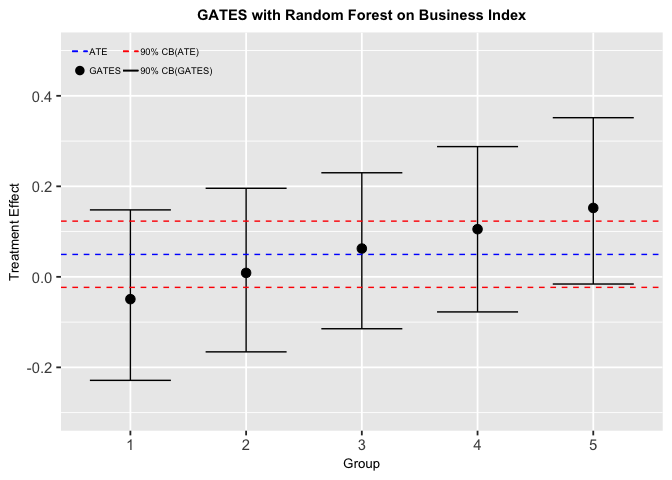
Figure5-2-1: Sorted Groups Average Treatment Effects for Business Index
The result shows that while the average treatment effect for all households is close to zero, there are signs of heterogeneity, at least for the fifth and the first group. This supports our hypothesis that the treatment effect is different for different groups of households. In addition, the result concludes that about half of the households have negative treatment effect, which might lead to the conditional treatment effect being close to zero on average.
In spite of the treatment being ineffective on average, the microfinance program could still make great impacts if the policy targets only the households that have positive treatment effect.
-
The Groups Separating Variables
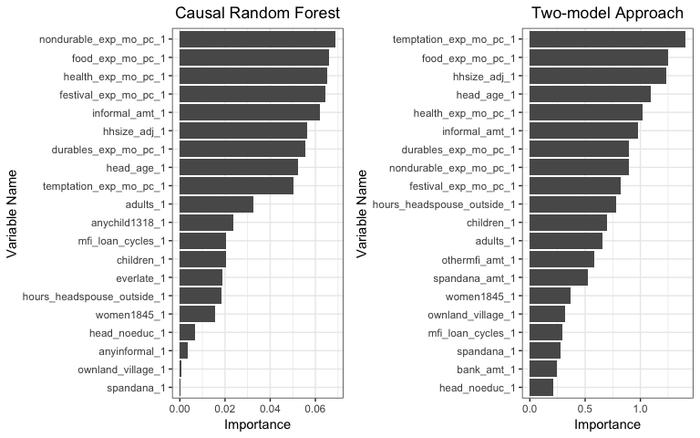
Figure5-1-2: left: Variable Importance predicted by Causal Random Forest; right: Vriable Importance predicted by Two-model Approach
Based on the results of the two methods, we can see that
food_exp_mo_pc_1, the household’s monthly expenditures on food per household member,health_exp_mo_pc_1, the household’s monthly health related expenditures per household member,hhsize_adj_1, the adjusted household size,informal_amt_1, the amount of informal loans a household has, are among the most important features that could determine how the treatment affects a household’s business situation.One interesting thing to notice is that expenses related variables dominates the results as most of them are highly important to separate households with high treatment effect. We could directly concludes from the result that household expenditures are important factors that determine the effectiveness of our treatment. However, the problem is that the relationship of expenditures and the success of business makes it difficult to exclude the possibility of endogeneity issue. Does the amount of expenditures affect how well the business improve from the treatment or are the changes in expenditures the results of changes in business status? In this case, the two effects needed to be separated in order to get reasonable inferences.
There are ways to deal with issues of endogeneity. One well known method is to construct instrumental variables to mitigate the problem. However, as a well defined instrumental variable could not be found in the dataset, this method could not be applied in this case. The viable albeit imperfect option left is to just delete those expenditures related variables. Hence for the following analysis, the dataset with expenditure variables (
nondurable_exp_mo_pc_1,health_exp_mo_pc_1etc) excluded will be used.
Business Index Without Expenditures Variables
target_index <- "biz_index_all_1"

endline1_biz_noexp <- endline1 %>%
  filter(total_biz_1 != 0) %>%  # filter only the household with a least on business
  select(everything(),
         -hhid,
         -contains("biz"),   # exclude business related variables
         -contains("exp"),   # exclude expenditures related variables
         -contains("index"), # exclude all index variables
         target_index)       # add back the target index variable
-
Heterogeneity of Treament Effect on Business Index
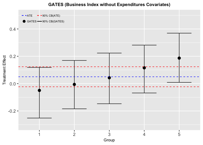
Figure5-2-1: Sorted Groups Average Treatment Effects for Business Index without expenditures variables
The result is similar to the above one (Business Index with expenditure covariates).
-
The Groups Separating Variables
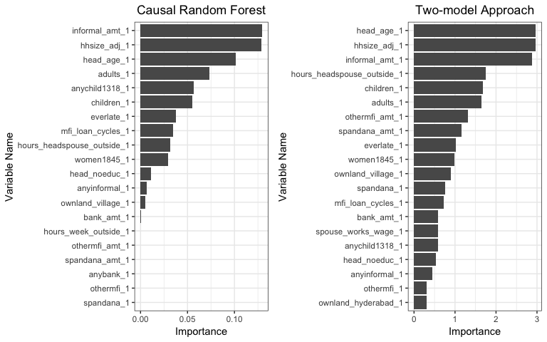
Figure5-2-2: left: Variable Importance predicted by Causal Random Forest; right: Vriable Importance predicted by Two-model Approach
After we exclude expenditure related variables, the results of the two methods are more aligned and the most important variables then become “The Amount of Informal Loans”, “Adjusted Household Size” and “Head Age”. In the following section we will discuss and try to find the optimum value for each feature.
-
Amount of Informal Loans
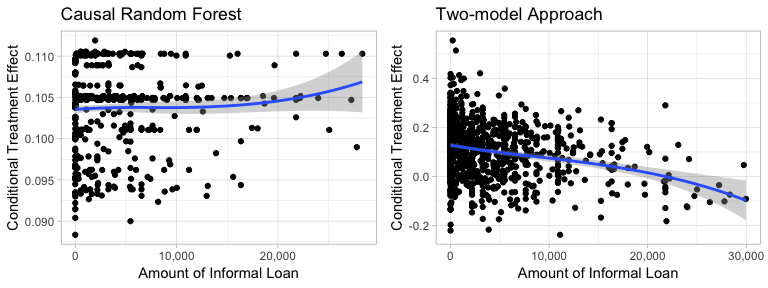
Figure5-2-3: Scatter Plot of Amount of Informal Loans to Predicted Conditional Treatment Effect
Based on the result of Causal Random Forest, we can see that there is no general pattern of how the amount of informal loans affect the predicted treatment effect. However, the result of Two-model Approach shows a slight trend that increasing the amount of informal loan will decrease the treatment effect.
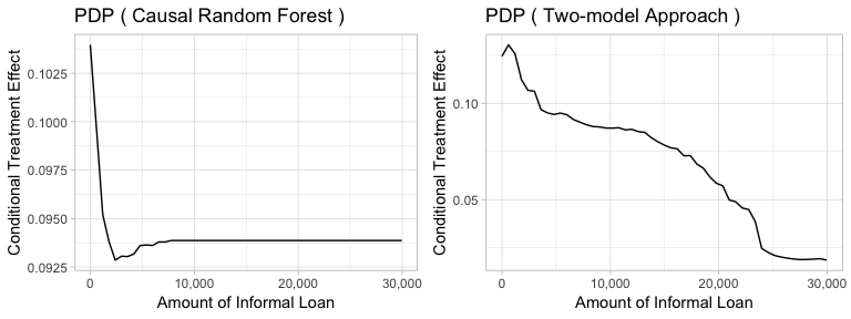
Figure5-2-4: Partial Dependence Plot of Amount of Informal Loans to Conditional Treatment Effect
Next, the partial dependence plots is used to find the critical values that lead to higher treatment effect. This time, both models predict that households with larger amount of informal loans tend to have lower treatment effect. And the optimal amount of informal loans should be close to zero.
-
Adjusted Household Size
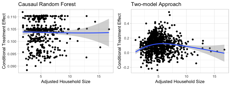
Figure5-2-5: Scatter Plot of Adjusted Household Size to Conditional Treatment Effect
We can see that while Causal Random Forest predicts no clear pattern of how adjusted household size affect conditional treatment effect. On the other hand, Two-model Approach indicates that households with adjusted household size being around 5-6 have relatively higher treatment effect.
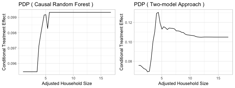
Figure5-2-6: Partial Dependence Plot of Adjusted Household Size to Conditional Treatment Effect
The partial dependence plots reflect the above results. Causal Random Forest tells us that once the adjusted household size is above 4, the conditional treatment effects become relatively stable. On the other side, Two-model Approach implies that there exists an optimal adjusted household size, which is around 4-5. And once the adjusted household size passes the threshold, the treatment effect starts to diminish.
-
Head Age
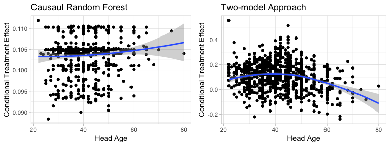
Figure5-2-7: Scatter Plot of Head Age to Conditional Treatment Effect
In the case of head age, the two methods suggest slightly different results. From the scatter plot, Causal Random Forest shows almost negligible pattern that increasing the head age increases the treatment effect. Yet Two-model Approach shows that as the head age increases, the treatment effect will first increase then decrease.
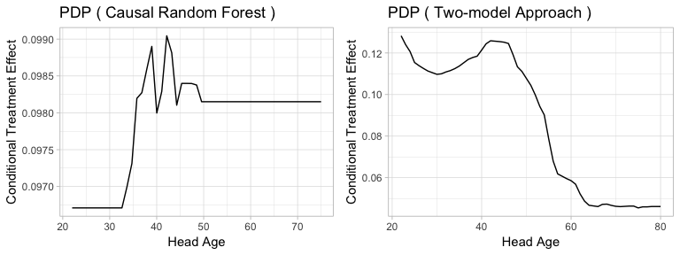
Figure5-2-8: Partial Dependence Plot of Head Age to Conditional Treatment Effect
Same as the scatter plots, the partial dependence plots also show somewhat contrasting results. Causal Random Forest indicates that as the head age increases, the treatment effect tends to increase, while Two-model Approach suggests the opposite. However, both methods suggest that there exists an optimal range, which is around 35-50. Both methods predicts that households with head age around 35-50 tend to have higher conditional treatment effect.
Women Empowerment Index
target_index <- "women_emp_index_1"

endline1_woemp <- endline1 %>%
  select(everything(),
         -hhid,
         -contains("index"), # exclude all index variables
         target_index)       # add back the target index variable
-
Heterogeneity of Treament Effect on Business Index
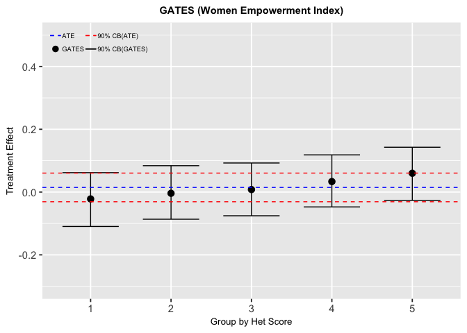
Figure5-3-1: Sorted Groups Average Treatment Effects for Women Empowerment Index
The GATES result shows little difference to the treatment effects across groups, and the overall average treatment effect is close to zero. This might conclude that the treatment effect on women empowerment index is homogeneous and the program did no significant impact on empowering women.
In this case, we could conclude that because of the homogeneity of the treatment effect, we cannot find features to target that could potentially increase the performance of the microfinance program.
However, since the first and the fifth groups are on the edge of the significance interval, we thought that it’s still worth to further investigate since the loan is given to women leading the women empowerment index an important target.
-
The Groups Separating Variables
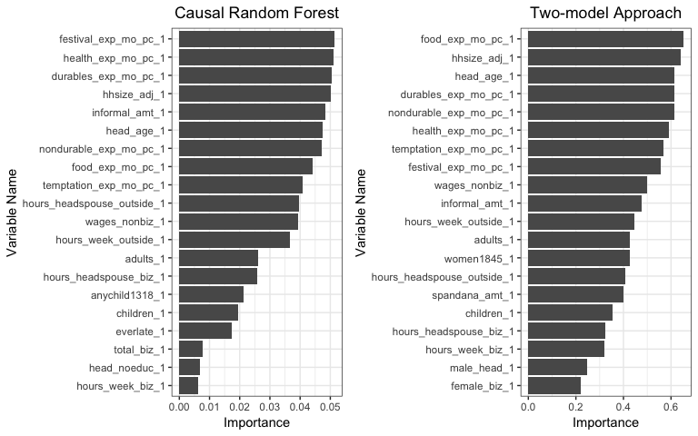
Figure5-3-2: left: Variable Importance predicted by Causal Random Forest; right: Vriable Importance predicted by Two-model Approach
In the case of women empowerment index, the results of variable importance produced by the two methods become fairly different from each other. In addition, none of the feature is significantly more important than the others. One of the reasons of this misaligned result could be because the differences between the high treatment effect group and the low treatment effect good are so small. Hence the two methods start to pick up noisy information that are actually not relevant.
Nonetheless, we are curious about whether we can still find the most efficient value of a given variable in this case. Therefore we pick
durables_exp_mo_pc_1, how much money a household spends on durable goods monthly per household member,hhsize_adj_1, the adjusted household size,head_age_1, the age of household head, to perform the following analysis. -
Durable Goods Expenditures
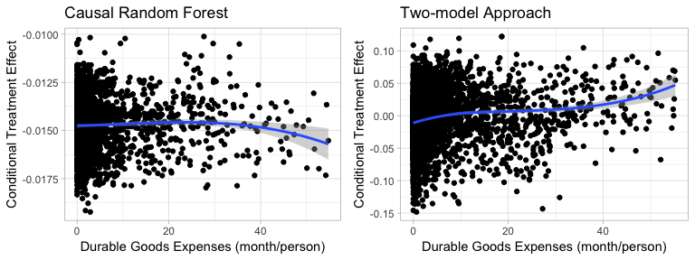
Figure5-3-3: Scatter Plot of Durable Goods Expenditures on Conditional Treatment Effect
While the Two-model approach shows that higher durable expenses lead to higher conditional treatment effect, the result of Causal Random Forest shows no significant pattern.
In addition, notes that Causal Random Forest always predict negative treatment effect, which means that our treatment will always hurt women’s well being in the area. Therefore we do not take the outcome for durables good into an account.
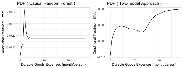
Figure5-3-4: Partial Dependence Plot of Durable Goods Expenditures to Conditional Treatment Effect
-
Adjusted Household Size
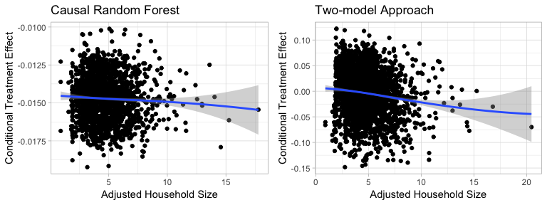
Figure5-3-5: Scatter Plot of Adjusted Household Size on Conditional Treatment Effect
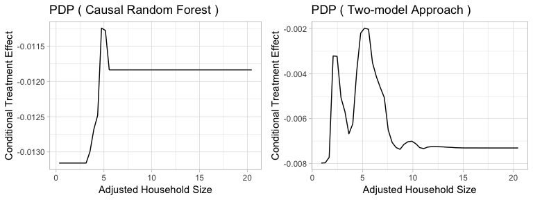
Figure5-3-6: Partial Dependence Plot of Adjusted Household Size to Conditional Treatment Effect
The patterns are similar in the two methods and partial dependence plots show that households with adjusted household size around 5 have relatively higher treatment effect. The difference is that Two-model approach shows two peaks as Causal Random Forest shows only one.
-
Head Age
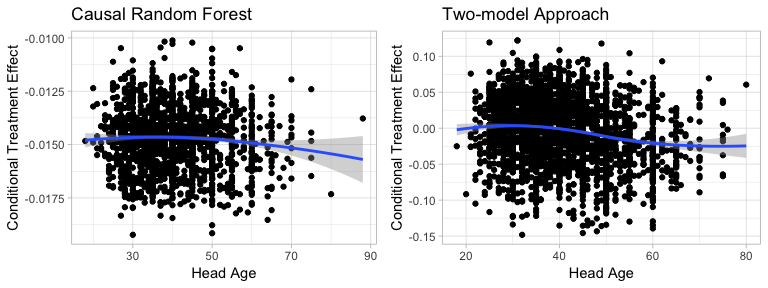
Figure5-3-7: Scatter Plot of Head Age on Conditional Treatment Effect
Scatter plots show no significant pattern of how head age influence conditional treatment effect.
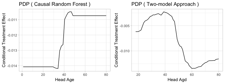
Figure5-3-8: Partial Dependence Plot of Head Age to Conditional Treatment Effect
The results of partial dependence plots show conflicting results. While Causal Random Forest predicts that higher head age leads higher conditional treatment effect, Two-model Approach predicts the contrasting result that households with lower head age will have relatively high conditional treatment effect. Again, this could be because the treatment effect in this case, on women empowerment index, is in fact homogeneous and the two methods are trying to solve a nonexistent problem. Hence they produce noisy results that cannot be interpreted.
Model Comparison
Measuring and comparing the performance of our two methods is not straightforward as calculating MSE (mean square error) or determining the accuracy. Since in real life causal inference problems, we do not have the true treatment effect. Then the above mentioned metrics can not apply under this circumstance as theyneed to compare the predicted value with the true value.
Usually the metric used to compare the performances of different uplift methods is Qini score, where the area under the incremental gains curve was measured. However, considering the target variables we selected in this project are continuous instead of binary, Qini score is not suitable in our case. There are ways to circumvent this issue. For example we could convert the numeric values into binaries based on some predefined thresholds that indicate whether or not a household “really” benefit from the treatment. However, defining the threshold without further information is problematic in practice. Hence at the end we did not take this approach.
The other comparing method is to use the transformed outcomes as “true” value and calculate the distance of predicted value and the transformed outcome (Hitsch & Misra 2008). This way the conventional error measurement, such as mean absolute error (MAE) and mean square error (MSE), could be implemented to assess the model performance. For this project we decided to use transformed outcome approach with mean square error as the error metric when comparing the performances of the two methods.
| Methods | Causal Random Forest | Two-model Approach |
|---|---|---|
| Business Index (without Expenditures Covariates) |
0.1500734 | 0.1372834 |
| Women Empowerment Index | 0.05090984 | 0.0476428 |
The results show that Two-model Approach is slightly better performing in both cases.
Interpretation And Policy Suggestions
Increase in informal loans decrease the positive treatment effect on business index, meaning that dealing with informal loans could be a suggestion to the microcredit institution. Different marketing strategies can be used and institutions can offer more suitable terms such as low interest rates on loans.
The other results related to the businesses were the optimal head age and household size which had affected more. These are around 5 for the household size and between 35-50 for the househead age. Besides, the optimal household size around 5 has also came up significant for the women empowerment index too. However, it would be a discriminatory policy to directly implement. Since the Reserve Bank of India prohibits banks from discriminating against customers on grounds of gender, age, religion, caste and physical ability while offering products and services (Kulkami 2014).
Conclusions
Both challenges addressed in the motivation part could be undertaken by the analysis.
By using uplift models which are Causal Random Forest and Two-model Approach the incremental effect of a treatment is captured and we tried to find the heterogeneity between subgroups whose business and women empowerment indexes are affected by the treatment. As a result, a clear heterogeneity has been found for the business index, could have not been found for the women empowerment index. In the case of Business Index, where heterogeneity is found, the results of two methods are quite similar in the sense that the important variables and their critical thresholds are very much alike. However, in the case of Women Empowerment Index, where heterogeneity is not clear, the results become very different. By interpreting the most important variables, which came up from the models and their significant value, some policies are suggested to microcredit institutions for better targeting.
References
-
Banerjee, Abhijit, Esther Duflo, Rachel Glennerster, and Cynthia
Kinnan. 2015. The Miracle of Microfinance? Evidence from a
Randomized Evaluation. American Economic Journal: Applied
Economics, 7 (1): 22-53.
https://www.aeaweb.org/articles?id=10.1257/app.20130533 -
Chernozhukov, V., Chetverikov, D., Demirer, M., Duflo, E., Hansen, C.,
& Newey, W. K. (2016). Double machine learning for treatment and
causal parameters (No. CWP49/16). cemmap working paper.
http://arxiv.org/abs/1608.00060 -
Chernozhukov, V., Chetverikov, D., Demirer, M., Duflo, E., Hansen, C.,
& Newey, W. (2017). Double/debiased/neyman machine learning of
treatment effects. American Economic Review, 107(5), 261-65.
https://www.aeaweb.org/articles?id=10.1257/aer.p20171038 -
Chernozhukov, V., Demirer, M., Duflo, E., & Fernandez-Val,
I. (2018). Generic machine learning inference on heterogenous
treatment effects in randomized experiments (No. w24678). National
Bureau of Economic Research.
https://www.nber.org/papers/w24678 -
Hitsch, Guenter J. and Misra, Sanjog, Heterogeneous Treatment
Effects and Optimal Targeting Policy Evaluation (January 28,
2018).
https://ssrn.com/abstract=3111957 -
Jacob, Daniel. (2018). Causal Inference using Machine Learning.
https://www.researchgate.net/publication/328686789_Causal_Inference_using_Machine_Learning -
Kulkami P., 2014. Five basic rights for bank customers laid down by
RBI. Retrieved from
https://economictimes.indiatimes.com/industry/banking/finance/banking/five-basic-rights-for-bank-customers-laid-down-by-rbi/articleshow/45584445.cms -
Mader, P. (2013). Rise and fall of microfinance in India: The Andhra
Pradesh crisis in perspective. Strategic Change, 22(1-2), 47-66.
https://pure.mpg.de/pubman/faces/ViewItemOverviewPage.jsp?itemId=item_1971501 -
Morrison, A., Breen, J., & Ali, S. (2003). Small business growth:
intention, ability, and opportunity. Journal of small business
management, 41(4), 417-425.
https://onlinelibrary.wiley.com/doi/abs/10.1111/1540-627X.00092 -
Radcliffe, N. J., & Surry, P. D. (2011). Real-world uplift
modelling with significance-based uplift trees. White Paper
TR-2011-1, Stochastic Solutions.
http://citeseerx.ist.psu.edu/viewdoc/download?doi=10.1.1.441.5361&rep=rep1&type=pdf - Strickland, J. S., 2014. Predictive Analytics Using R
-
Van Stel, A., Carree, M., & Thurik, R. (2005). The effect of
entrepreneurial activity on national economic growth. Small
business economics, 24(3), 311-321.
https://link.springer.com/article/10.1007/s11187-005-1996-6 -
Wager, S., & Athey, S. (2018). Estimation and inference of
heterogeneous treatment effects using random forests. Journal of
the American Statistical Association, 113(523), 1228-1242.
https://www.tandfonline.com/doi/abs/10.1080/01621459.2017.1319839