Matching Methods for Causal Inference: A Machine Learning Update

Authors: Samantha Sizemore and Raiber Alkurdi

Introduction

Practitioners from quantitative Social Sciences such as Economics, Sociology, Political Science, Epidemiology and Public Health have undoubtedly come across matching as a go-to technique for preprocessing observational data before treatment effect estimation; those on the machine learning side of the aisle, however, may be unfamiliar with the concept of matching. This blog post aims to provide a succinct primer for matching neophytes and, for those already familiar with this technique, an overview of how state-of-the-art machine learning can be incorporated into the matching process. In addition, we provide a replicable coding excursion that demonstrates how different matching methods perform on various data generating processes and discuss if any one method can be deemed “better” for a certain type of dataset.

By the conclusion of this read, you should have a clear grasp of:

• the statistical assumptions that make matching an attractive option for preprocessing observational data for causal inference,
• the key distinctions between different matching methods, and
• recommendations for you to implement matching, derived both from our analysis and from contemporary academic research on matching.

Tables of Contents

1. Matching Motivation: Observational Studies and the Fundamental Problem in Causal Inference
2. Matching Motivation: Definition, History and Situating Matching within the Canon of Causal Inference
3. Matching Statistical Framework and Assumptions
4. The Matching Family Tree: Stratification, Modeling, and Machine Learning Methods
5. Outline of Our Methodological Approach for Comparing Matching Methods
6. Synthetic Data Generating Process to Generate 6 Datasets
7. Evaluation Metrics: Known ATT / Mean Absolute Error
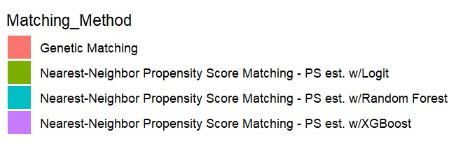
8. Match (and Estimate ATT) with 5 Matching Methods:

• Coarsened Exact Matching
• Nearest-Neighbor Propensity Score Matching, with Propensity Score estimated with Logistic Regression
• Nearest-Neighbor Propensity Score Matching, with Propensity Score estimated with Random Forest
• Nearest-Neighbor Propensity Score Matching, with Propensity Score estimated with XGBoost
• Genetic Matching

9. Compare Performance in estimating ATT of 5 Matching Methods on 6 Datasets
10. Conclusions & Recommendations: Academic + Results from Our Experiment
11. References

1. Matching Motivation: Observational Studies and the Fundamental Problem in Causal Inference

Before delving into the details of matching, we provide a brief refresher on the fundamental problem in causal inference with observational studies. The LaLonde dataset, which is pre-loaded in RStudio, provides such motivation: it includes characteristic background data on individuals, some of whom were selected for enrollment in a job training program. The training program was operation in ten states in the United States by the Manpower Demonstration Research Corporation, and specifically targeted recently unemployed women, ex-drug addicts, ex-criminal offenders, and high school dropouts. [1] The dataset provides the annual income for enrollees and non-enrollees in the year subsequent to training. A naïve difference-in-means estimation of the treatment effect of job training (i.e. the difference in average income of treated and control individuals) finds that those enrolled in the program earned $635 less than those who did not have job training. [2]

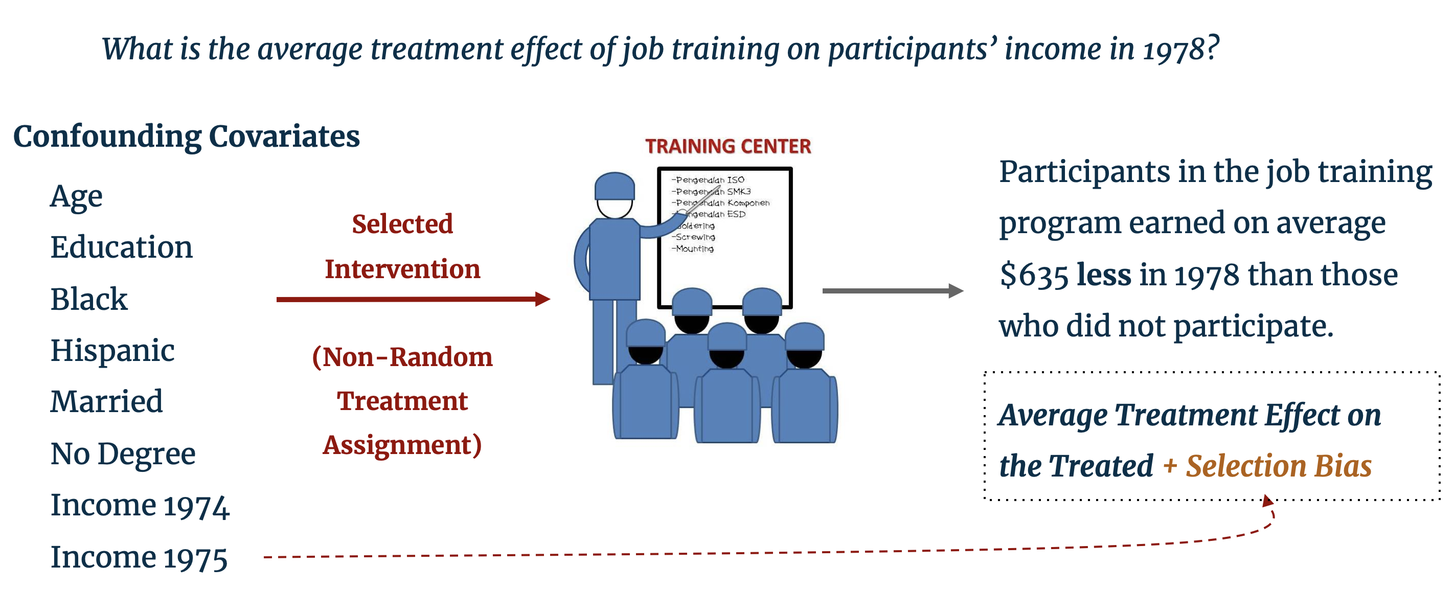
As perceptive statisticians, instead of concluding that the training program had a negative impact on trainees’ earning potential we should look to the treatment assignment mechanism. In the LaLonde study, individuals were selected into treatment specifically because of their low earning potential and therefore systematically differ from those in the control group who were not selected for job training. Clearly, the characteristics that determine the probability of selection into treatment are biasing the estimated treatment effect. The training program may well have had a positive effect on trainees’ income, but, as our control and treatment groups are fundamentally different, the effect of the training program is obfuscated by this selection bias. The problem of selection bias extends beyond the social sciences and is often encountered in the business world; for example, do customers who earn a coupon for spending a certain amount in an online shop go on to spend more because of the coupon or because of their background characteristics that prompted them to shop online in the first place?

The gold standard for disentangling these channels of causality is to conduct a randomized trial which utilizes a randomized treatment assignment mechanism. Provided that we have a sufficiently large sample size, random treatment assignment should “successfully balance subject’s characteristics across the different treatment groups” [3] as the treated and control groups should be only “randomly different from one and other on all background covariates, both observed and unobserved.” [4] (In business analytics, this implemented as A/B Testing.) Randomization ensures that our treatment and control groups do not systematically differ, and therefore removes this selection bias.

It is, however, often unethical or costly to play such a heavy hand in treating individuals at random. For example, we cannot force some individuals to smoke to find the effect of smoking, and perhaps not treating some customers may incur a cost to a business’s bottom line. Furthermore, we may be dealing with data after-the-fact where we cannot control the design of the experiment, but rather passively observe what happened. Save resorting to a time machine to see “what would have happened” to the treated individuals had they not been treated, researchers are frequently confronted with observational data like the LaLonde dataset, mired with selection bias and incomparable treatment and control groups.

2. Matching Motivation: Definition, History and Situating within the Canon of Causal Inference

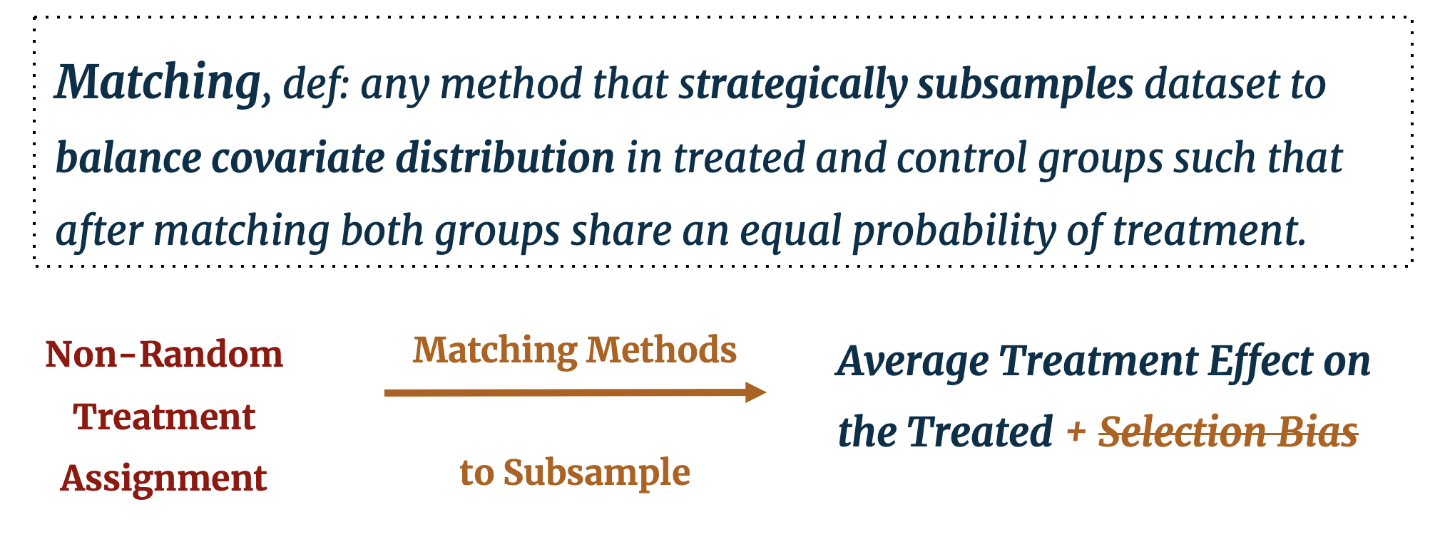
First, what is matching? Matching as it is known today is one of several statistical techniques that emerged in the 1980s with the aim of estimating causal effects. [5] Matching can be defined as any method that “strategically subsamples” a dataset [6], with the aim of balancing observable covariate distributions in the treated and control groups such that both groups share an equal probability of treatment. Alternatives, or complements, to matching include: “adjusting for background variables in a regression model; instrumental variables; structural equation modeling or selection models.” [7] An important distinction from other statistical approaches is that matching is only the first step in a two-step process to estimate the treatment effect. It prepares the data for further statistical analysis, but it is not a stand-alone estimation technique in and of itself. (In machine learning terms, it is part of the data preprocessing step not the modeling step.) Matching is followed by difference-in-average estimation (assuming sufficient covariate coverage), linear regression, or any other modeling method. Proponents of this technique proclaim that one of the greatest conveniences to using matching is precisely this flexibility: preprocessing with matching can be followed by “whatever statistical method you would have used without matching.” [8]

While there is an interesting pedagogical debate in causal inference academia around how matching should be taught [9], there is a general consensus that matching should be understood as a complement to other approaches instead of being at odds with them (i.e. practitioners should consider not matching or regression, rather matching and regression). [10] Not every causal inference observational study uses matching, and it should be noted that it is not the ambition of this project to compare matching against other causal inference approaches that do not use matching. We aim, rather, to provide some brief guidelines around when it may be useful to use matching as a preprocessing step and focus the bulk of our analysis on illuminating the differences between matching approaches and their effectiveness on different data generating processes.

Since the first publications by Rosenbaum and Rubin in the 1980s [5], dozens of matching methods have been proposed across various disciplines. The evolution of matching has developed from “exact” matching to matching on propensity scores, to more novel “algorithmic matching” approaches that incorporate machine learning searches for optimal matching outcomes. The algorithmic approaches are innovative in that search for the optimal number of control cases to be matched to each treated unit and/or search for optimal weighting of matched control units to each treated unit. [11] More on this distinction will be presented later.

How does one implement matching? Whether the matching method is standard or algorithmic, each approach follows the same basic process: define a metric of “closeness”, match control to treatment observations 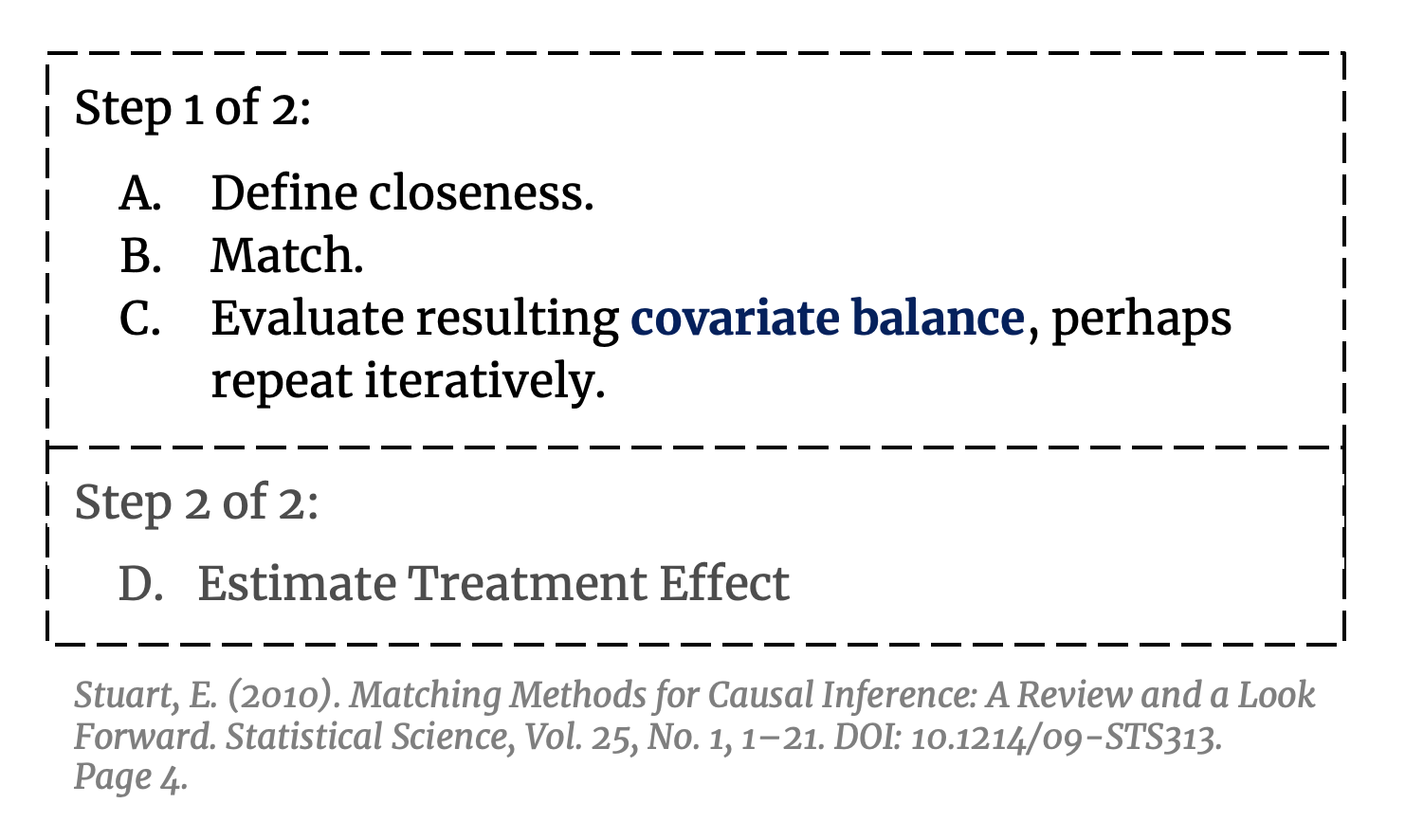based on this metric, and discard unmatched observations. [12] Algorithmic matching methods go on to evaluate the resulting covariate balance and repeat the matching process until an optimal covariate balance is achieved. The proliferation of distinct matching methods emerged from various permutations of A/B (e.g. how to define a good match, how to use the matches (one, construction, average, or weighted), what order to match on, how many observations to discard, if matching should be done on only “important” covariates, etc.). As the purpose of this project is to evaluate matching methods, we will focus here solely on matching (Step 1 of 2).

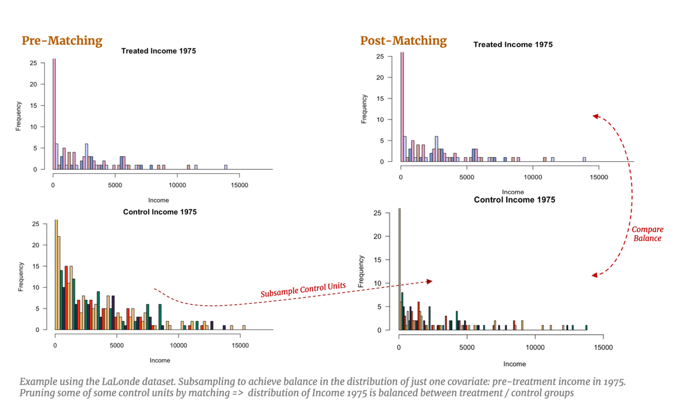
The ultimate goal of causal inference is an unbiased estimation of the treatment effect, while the main metric of interest in evaluating the effectiveness of matching is the resulting covariate balance between the treatment and control groups. 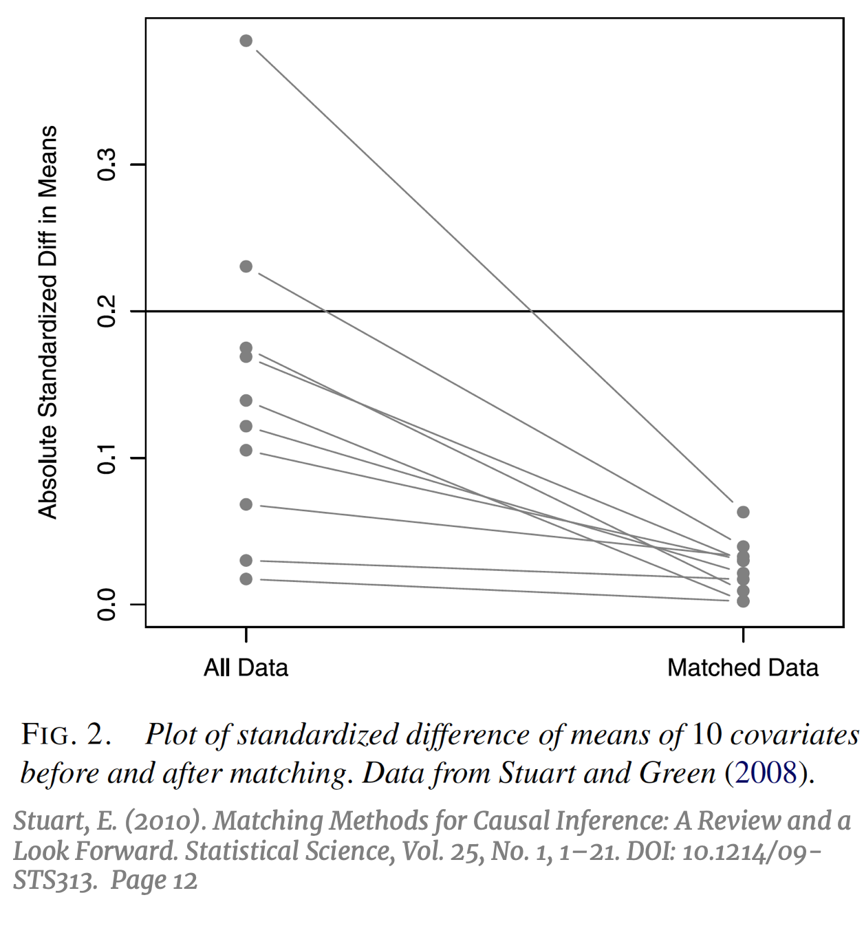The prior should beget the former, if done correctly. It is important to note that the use of the term “balance” in matching does not refer to the standard concept of balance in machine learning; typically, a “balanced” dataset is one with an equal number of observations across all categories of the outcome variable Y, or an equal number of observations across all treatment groups. Balance in matching refers to a different concept that can be defined as the treatment and control groups having “the same joint distribution of observed covariates.” [13] To avoid confusion, this particular concept of balance in matching will be referred to subsequently as “covariate balance”. Subsampling by matching to achieve covariate balance might result in a balanced number of treatment and control units, but not necessarily. The success of matching to balance the covariate distributions can be visualized by comparing the absolute standardized difference in means of each covariate, pre and post-matching [14] (right).

Let’s also consider a practical example with the LaLonde study and imagine, for simplicity, we have only one confounding covariate: pre-treatment income in 1975. Covariate balance would imply subsampling the control units such that the distribution of pre-training income for the control group matches the distribution of pre-training income for the treated group. With multivariate data, this example would be extended to subsample so that all observable covariates are simultaneously balanced, resulting in a balance of the multivariate distributions. [15] Naturally, this subsampling allows for a fairer comparison between our treated and control groups: if covariate balance is achieved, estimating the effect of training should capture the effect of treatment alone. This task becomes more difficult with higher dimensional data which we will explore below.

But how do we go about pruning our dataset to achieve this covariate balance? A perhaps overly reductive, yet intuitively useful, way to conceptualize matching is the simple one-to-one approach: we identify a treated individual and review the pre-treatment characteristics that affects their probability of treatment (years of education, annual income, etc.) and search our control group for an individual with a similar background. The control individual identified should look very much like she would have been treated, however in the end she was not. Thus, she serves as an excellent counterfactual for the treated individual whose non-treatment outcome is unobserved. We can then estimate the individual treatment effect for this treated individual using the observed outcome of the control individual. Provided we find good matches for the remaining treated individuals, we can also estimate the overall Average Treatment Effect on the Treated (ATT).

This is an opportune moment to formalize some of the statistics terminology around treatment effect estimation and to define the statistical assumptions that make matching an effective preprocessing intervention.

3. Matching Motivation: Statistical Framework and Assumptions

We employ the framework from the Rubin Causal Model [16], an oft-cited rubric for causal effect estimation in observational studies. Here, we use notation from King, 2011 [17]:

• For unit i (i =1, …, n) Ti denotes the treatment variable such that Ti = 1 indicates the individual was treated and Ti = 0 indicates the individual was not treated.
• Let Yi (t) for (t = 0,1) denote the value of the outcome variable. For each observation i, only Yi (0) or Yi (1) is observed but not both.
• Let X denote the vector of pre-treatment variables.
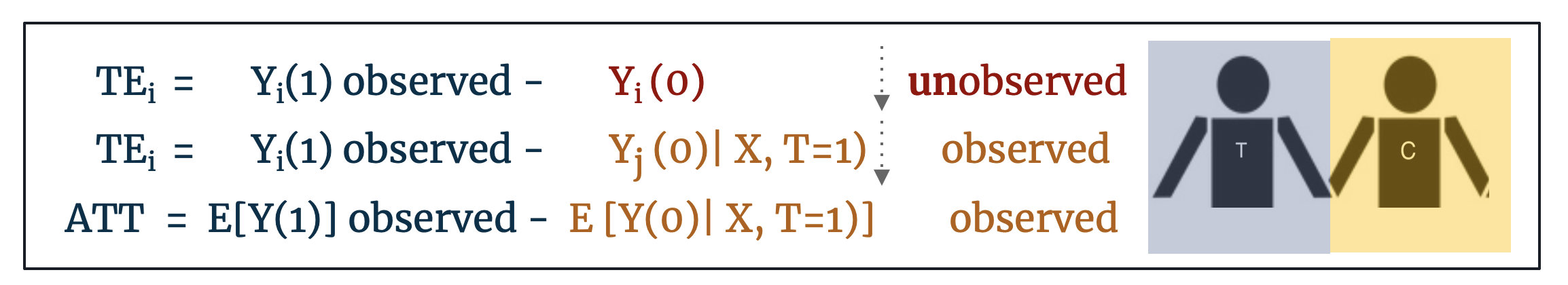
• Let TEi denote the individual treatment effect defined as: TEi = Yi (1) - Yi (0). For a treated individual, only Yi (1) is observed. If we find a control individual such that Xi = Xj, we estimate TEi = Yi (1) – Yj (0)

Most frequently, matching is employed as a first step in estimating the Average Treatment Effect on the Treated (ATT) defined as: E [Y(1) – Y(0) | X, T=1]. The ATT matches control units to treated units on the basis of Xi ≈ Xj. If control units are matched exactly to treated units such that Xi = Xj then we can say that this is the estimated Average Treatment Effect (ATE) where ATE = E [Y(1) - Y(0)]. Alternatively, and less frequently invoked, if treated units are matched to control units then we have the estimated Average Treatment Effect on the Controls (ATC) defined as: E [Y(1) – Y(0) | X, T=0]. [18]

The distinction between ATE and ATT is important: if we can match treated units to control counterfactuals that are identical on all observables then we can conclude that this is the estimated ATE for the population, but most often this exact matching is not possible. If our found control counterfactuals are less-than-perfect matches on the observables (Xi ≈ Xj), we should conclude only that this is the average treatment effect on the treated (ATT) as the treated outcomes are the only outcomes we actually observe. Further, if matching goes so far as to prune treated units for which there are no good control matches, conclusions should be restricted to Feasible Sample Average Treatment Effect on the Treated (FSATT). [19]

Causal inference has been increasingly focused on observational data with heterogenous treatment effects. This can be understood as the treatment effect varying across different sub-groups of the population; for example, job training may result in a $5,000 increase in annual salary for those with a college degree, but only a $2,000 increase for those without a college degree. This heterogeneity across X can provide powerful insight for researchers, policymakers, and marketers alike. If our treatment has little effect on one sub-group, resources can be better applied to the group with the largest positive treatment effect.

Because unit-level matching preprocesses the dataset with the aim of 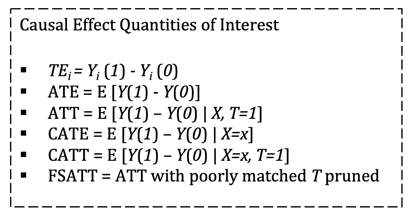balance across sub-groups, it is a natural first step in estimating the Conditional Average Treatment Effect (CATE) when we suspect heterogeneity of X results in heterogeneity in the treatment effect. CATE is defined as E [Y(1) – Y(0) | X=x]. If a matching method matches a control unit to a treated unit to achieve covariate balance on the unit level, then estimation of TEi and CATE are possible. However, if the matching method seeks to match control units to treated units to achieve covariate balance on the group level (as in propensity score matching) then individual matched pairs may not be similar across X and it may not be possible to calculate TEi or CATE, especially in high dimensions. [20]

As commented previously, not all causal inference studies use matching so how should a researcher decide if it is appropriate to use matching for a particular dataset and research question? To understand the appeal of matching, let’s first outline the assumptions required for unbiased treatment effect estimation and some common problems that may arise in their violation. Here again we use the Rubin Causal Model, summarized by Lam, 2017 [21]:

1. Stable unit treatment value assumption (SUTVA) states that the treatment of one unit does not affect the potential outcome of other units (i.e. there are no network effects). It further assumes that the treatment for all i are similar. (In the LaLonde study this means that the job training program was more or less the same quality for all individuals across the ten states where it was administered).

2. Ignorability assumes that the treatment assignment is independent of the potential outcome, Y(1), Y(0) ⟂ T. This assumption, sometimes referred to as Unconfoundedness or selection on observables in econometrics [22], is assumed to hold in randomized trials. With observational studies, however, one can never be completely certain that this holds. [23] The most common violation of ignorability is omitted variable bias where an unidentified variable is affecting both the probability of treatment and the outcome, thereby biasing the treatment effect estimate. The typical way to address omitted variable bias is to identify and include all variables that make the treatment assignment independent of the outcome such that conditional ignorability, defined as Y(1), Y(0) ⟂ T | X, holds.
   
   A natural way to think about conditional ignorability is to assume we can control for all confounding covariates so that, “any two classes at the same levels of the confounding covariates (…) have the same probability” of receiving the treatment. [24] In reality, perfect conditional ignorability is an elusive goal with observational studies. The best researchers can do is take care to identify and include all possible confounding covariates.

3. While perhaps a leap of faith, let’s assume that SUTVA and conditional ignorability hold. We are still confronted with a third problem: lack of overlap and imbalance between the treated and control groups. Gelman’s graphs below illustrate this problem clearly.

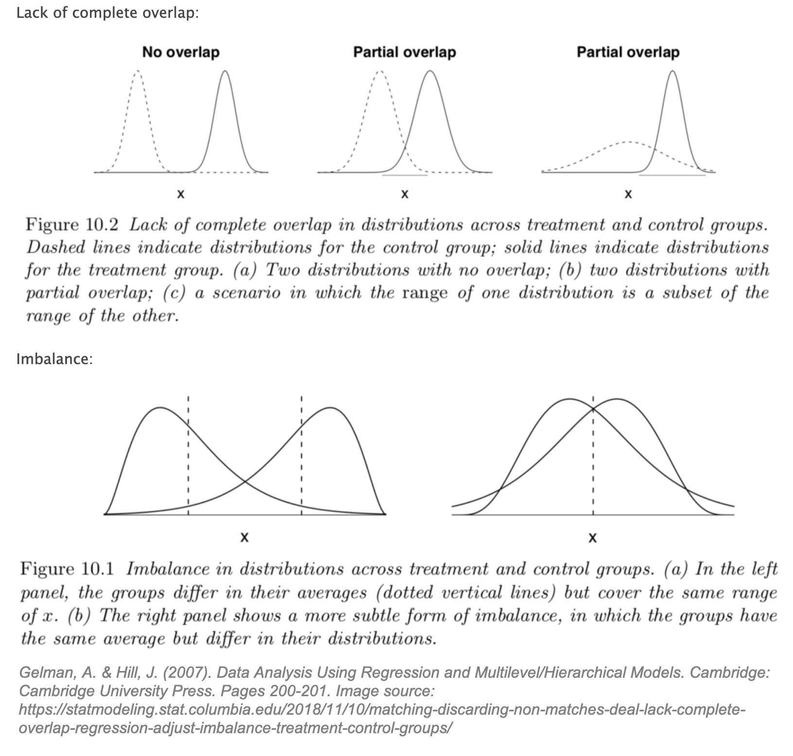
Gelman states that lack of overlap forces us to, “rely more heavily on model specification and less on direct support from the data.” [25] For causal inference, this means we may be missing counterfactuals and therefore force our model to “extrapolate beyond the support of the data”. [26]

This extrapolation is a slippery slope into model dependence, or differing estimates of the treatment effect with different model specifications. [27] Estimates of the treatment effect that are heavily model-dependent show only that the researcher, however well-intentioned, was able to find a model “consistent with the author’s prior expectations.” [28] Matching is a preprocessing step that reduces model dependence as it restricts the dataset to areas of overlap, thereby reducing the parametric modeling assumptions required in Step 2 of 2 (modeling to estimate the treatment effect). Better overlap results in improved robustness in causal effect models and estimates.

In Rubin’s Causal Model, the overlap assumption (also referred to as common support) is defined as: 0 < Pr (T = 1 | X) < 1 for all i. An intuitive way to think about overlap is to consider the opposite extreme: if Pr (T = 1 | X) = 1 for all i then all units would be treated, and no possible control counterfactuals would exist. We need to assume that for a given individual, conditioned on X, there exists the possibility of not being treated. [29] If this assumption does not hold, there could be “neighborhoods of the confounder space” where there are treated units for which no appropriate control counterfactual is available. [30] If full overlap is assumed to hold, then conditional ignorability can be upgraded to a stronger assumption, strong ignorability defined as Y(1), Y(0) ⫫ T | X.

Finally, it is important to address that matching methods inherently discard, or weight to zero, un-matched observations thus reducing the available sample size. Standard statistical assumptions dictate that a smaller sample may increase the variance of our estimates; therefore, the claim that matching can improve model robustness by down-sampling may seem counterintuitive. Sekhon, 2008 [31] citing Rosenbaum, 2005 [32] addresses this concern:

“Dropping observations outside of common support and conditioning…helps to improve unit homogeneity and may actually reduce our variance estimates (Rosenbaum 2005). Moreover, as Rosenbaum (2005) shows, with observational 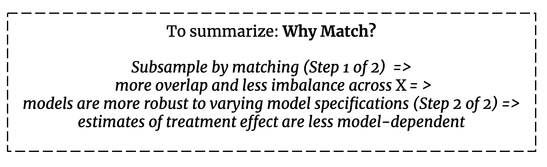data, minimizing unit heterogeneity reduces both sampling variability and sensitivity to unobserved bias. With less unit heterogeneity, larger unobserved biases need to exist to explain away a given effect. And although increasing the sample size reduces sampling variability, it does little to reduce concerns about unobserved bias. Thus, maximizing unit homogeneity to the extent possible is an important task for observational methods.”

At this point, we hope that the statistical basis of matching is evident. However, faced with dozens of matching methods how should you choose which approach is right for your dataset? Let’s outline and compare some of matching methods available.

4. The Matching Family Tree

Up until this point, our reference to matching’s goal of covariate balance has been intentionally over-simplified: it is easy to understand that subsampling to the dataset can result in a fairer comparison between the treatment and control groups. In practice, however, we are often faced with high-dimensional covariate spaces and continuous variables which make matching and covariate balance across all of X difficult. Matching approaches can be broadly divided into two groups, with this covariate dimensionality in mind: Stratification techniques can be used for low-dimensional datasets, but we must resort to Modeling through propensity scores or the like for higher dimensions. We provide a brief explanation of the differences in these approaches below and include more detailed exploration of the methods highlighted in green in the subsequent coding section.

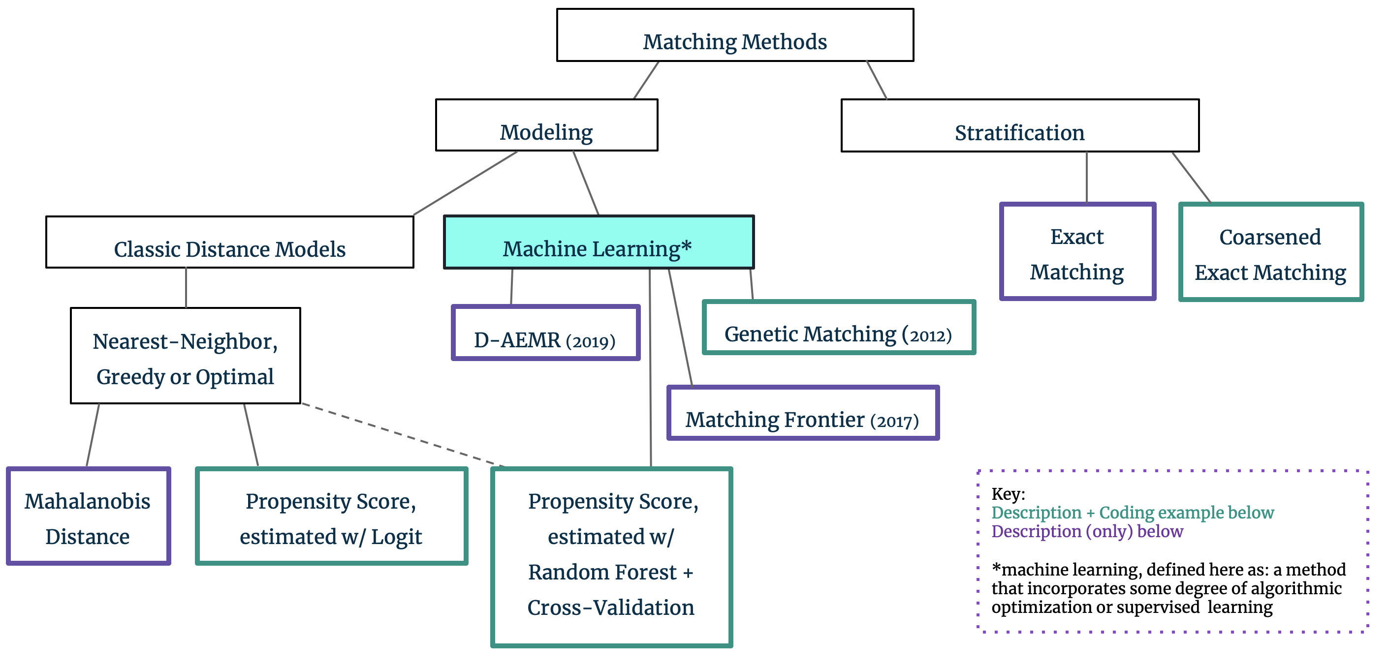
Stratification: Exact Matching and Coarsened Exact Matching

Preprocessing the data through stratification aims to replicate a controlled randomized trial by matching control and treated units in “bins” that represent all possible combinations of the observable covariates. “Perfect stratification of the data [means that] individuals within groups are indistinguishable from each other in all ways except for (1) observed treatment status and (2) differences in potential outcomes that are independent of treatment status.” [33]

Exact Matching
If there is sufficient overlap to have the same number of treated/control units in each bin, then exact matching can be implemented. Recalling the LaLonde study, if the observable covariates are simply college education (Yes/No) and income (High/Low), subsampling by one-to-one exact matching would mean placing all treated units in their respective bins (college/high income, college/low income, no college/high income, and no college/low income) and placing the same number of control units that meet the criteria in these same four bins. For a low-dimensional dataset exact matching should be the first choice: it is a simple and powerful method for pruning the dataset and balancing covariates in the treated/control groups.

Unfortunately, its simplicity also makes it unscalable for datasets with continuous variables or high-dimensional covariate spaces where exact matching would result in many empty bins. For example, if we attempt to match on college education (Yes/No) and 100 other categorical variables we are likely to have many bins with no treatment or control observations; similarly if we attempt to match on college education (Yes/No) plus income as a continuous variable from $0 to $50,000 we would have 100,000 (2x50,000) potential bins and likely insufficient matches. Coarsened Exact Matching, Mahalanobis Distance Matching and Propensity Score Matching are all techniques developed to deal with this continuous variable and/or high-dimension paradigm.

Coarsened Exact Matching (CEM)
CEM starts by transforming continuous variables into categorical variables. This technique in the machine learning is often referred to as discretization, or any process that converts a continuous variable into a finite number of categories, bins, features, etc. Invoking the mini-LaLonde example above, if the income variable is coarsened from a continuous scale into Low/Medium/High our matching problem is more manageable: instead of matching on 100,000 (2x50,000) bins, we now have only 6 (2x3) bins to fill with treatment/control individuals. After ‘filling’ the bins, “control units within each [bin] are weighted to equal the number of treated units in that stratum. Strata without at least one treated and one control are weighted at zero, and thus pruned from the data set.” [34]

Provided that exact matching is possible after coarsening, then CEM should take priority over other matching techniques that rely on modeling. CEM, and other Monotonic Imbalance Bounding (MIB) techniques, are preferred over matching by modeling (e.g. propensity score) as they more closely approximate randomized block experimental design. [35] If exact matching is not possible after coarsening, then further modeling techniques must be used however CEM can still be used as a first step preceding matching by propensity score. [36] Situations where CEM would be inappropriate are where, even after coarsening, there are many empty bins (either lacking a found counterfactual control or a treated unit) and pruning would lead to excessive reduction of the dataset. For additional details and implementation of this method, see Section 8 below.

Modeling: Mahalanobis Distance Matching and Propensity Score Matching

Mahalanobis Distance Matching (MDM)
For higher dimensional datasets where CEM is not appropriate, matching through modeling is required. Each of these approaches applies a linear transformation to the data for more effective matching. [37] Mahalanobis Distance Matching (MDM) 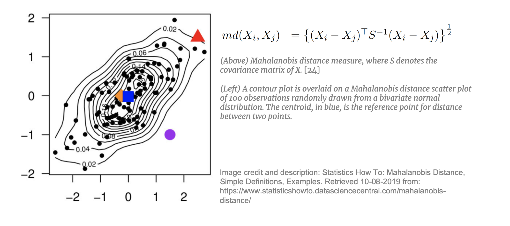takes each treated unit and, using the estimated Mahalanobis distance, matches it to the nearest control unit. Mahalanobis distance is mapped in an n-dimensional space and is appropriate for datasets with many continuous, potentially correlated, variables. MDM is preferred to simple Euclidean distance as it is weighted by the covariance matrix of X thereby taking into account the correlations between the variables. MDM is not, however, effective if the dataset contains covariates with non-ellipsoidal distributions (i.e. not normally- or t-distributed). [38] In addition, MDM in not appropriate for very high dimensions. Mahalanobis distance, “regards all interactions among the elements of X as equally important” [39] and with high-dimensional data this n-dimensional space becomes increasingly sparse [40] making it difficult to find an appropriate neighbor to match to.

Propensity Score Matching (PSM)
Matching on the propensity score is the most commonly used approach across the social sciences. As of 2018, it is estimated that over 93,000 published articles utilized some variant of PSM. [41] This popular technique addresses the main short coming of the previously outlined approaches. With exact matching, CEM and MDM the inability to find good counterfactual “twins” in the 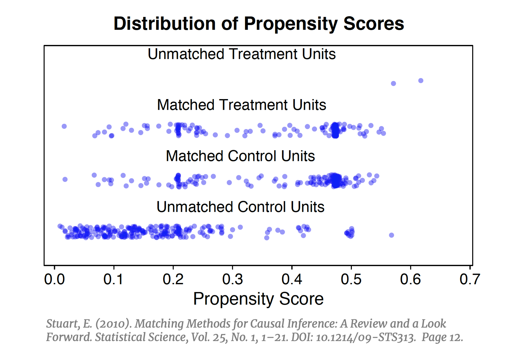dataset becomes increasingly difficult in higher dimensions and necessitates some way to reduce the dimensionality of the data. PSM does exactly this: instead of matching units on all X, it collapses the covariate space into one variable defined as the probability of being treated, conditioned on X. After calculating the propensity score, instead of trying to fill n-bins we can simply match units within strata of the propensity score (e.g. if strata .40-.60 has five treated units, find five control units with scores in this strata), and instead of finding nearest neighbors in a sparse n-dimensional space we need only to find nearest neighbors on a unidimensional plane. If implemented successfully, PSM should result in a balanced distribution of propensity scores in the treated and control groups (left).

PSM is most commonly implemented by:1) Estimating the propensity score through logistic regression, and 2) Matching control units to the closest treated unit(s) and discarding non-matched controls. It is the discretion of the analyst to determine if only one control should be matched to each treated, or if multiple control units should be matched to each treated unit. Standard nearest-neighbor matching is known as Greedy Matching as it matches control units to treated units one-by-one and without replacement. In contrast, Optimal Matching looks at the matching problem holistically by finding “the matched samples with the smallest average absolute distance across all the matched pairs.” [42] To match units on a unidimensional plane, it is common to plot a Gaussian distribution over treated observation and find the control unit(s) closest to the median. For example, below six potential control units are considered for matching to one treated unit; two are near the center of the distribution so we average their Y(0) to create the counterfactual outcome and can then calculate the TEi for the treated unit.

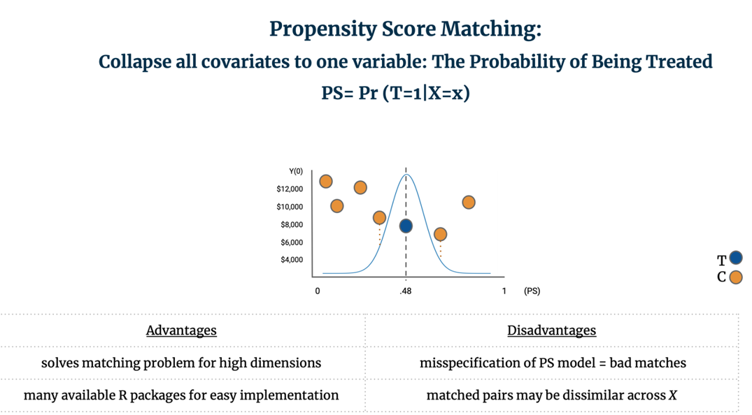
PSM solves the matching problem for high dimensional data and is easily implemented. It is important to note however that PSM results in matched pairs that are not necessarily similar across all of their covariates; rather, the goal of PSM is that the subsampled treatment and control groups are similar to each other on average across all of X. [43] Further, misspecification of the propensity score model can lead to bad matches. [44] For additional details and implementation of this method, see Section 8 below.

Machine Learning Modeling: Matching Frontier, D-AEMR, Genetic Matching, and Nearest-Neighbor PSM w/ Random Forest

The methods outlined so far were first proposed in the 1980s with tweaks and updates throughout the years. In recent years, novel approaches have been published with increasing frequency. These approaches utilize some degree of algorithmic optimization or supervised machine learning concepts to optimize individual matches, overall covariate balance, and/or the propensity score model itself. We provide summaries of Matching Frontier and D-AEMR, and summaries plus code for PSM with Random Forest and Genetic Matching.

Matching Frontier Matching Frontier, a package in RStudio [45], was developed by Gary King and colleagues to address a fundamental concern in matching: down-sampling improves covariate balance but may prune too many observations from the dataset. [46] This can be interpreted as a standard bias-variance trade-off: poor covariate balance can lead to biased causal effect estimates but pruning too many observations can increase the variance of the estimates. The Matching Frontier algorithm lets users define their metric of imbalance (difference-in-means or L1), and then plots the level of imbalance against the number of observations pruned. For a given number of observations pruned, the frontier indicates the lowest possible level of imbalance for a dataset of that size. Below, King applies this frontier to the LaLonde study using difference in scaled means (right) and LI (left) as the metrics of covariate imbalance. L1 is a difference-in-means estimate of the treatment and control multivariate histograms. [47] He illustrates how the frontier evolves as control units are matched, and others pruned:

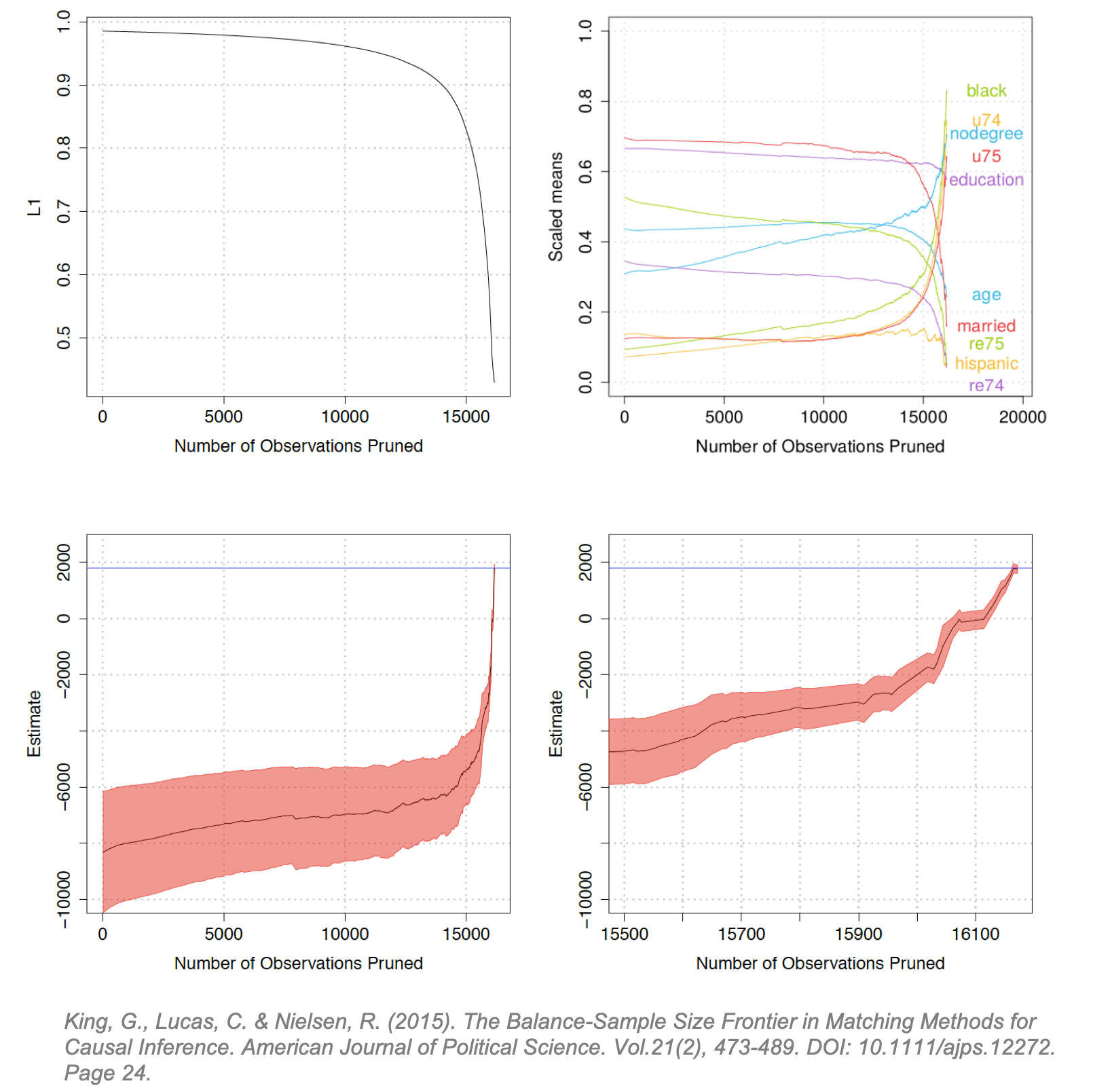
The upper-left diagram shows the inflection point at which pruning starts to reduce covariate imbalance (around 14,000). The upper-right diagram illustrates how this same inflection point affects the difference-in-means for each covariate. (Interestingly, at the same inflection point balance increases for some covariates and decreases for others.) The lower diagrams plot the estimated FSATT and “Athey-Imbens model dependence intervals”. (These intervals are proposed in Athey and Imbens (2015) and give an indication of model dependence. [48]) The lower-right diagram zooms into the tail-end of the lower-left diagram showing the inflection point where pruning precipitously reduces the dependence interval. The blue line is the true treatment effect. (The LaLonde study was conducted as both an observational study and a randomized trial so the blue line can be considered the true known TE resulting from the trial. [1])

The Frontier does not explicitly show if and where an increase variance in the FSATT begins as pruning progresses, but it can serve useful to determine if pruning will reduce imbalance and decrease model dependence and if so at which point. In doing so, it algorithmically solves the joint optimization problem of decreasing imbalance while maintaining the largest possible subsampled dataset. (King argues that typically, researchers are forced to manually optimize balance while algorithmically optimizing sample size or vice-versa. [49]) The upper-left and lower-right demonstrate that for the LaLonde study, pruning monotonically decreases covariate imbalance and model dependence. If we imagine this line fluctuating, the usefulness of the Frontier is more apparent.

Genetic Matching
Genetic Matching utilizes a genetic algorithm commonly employed in machine learning prediction tasks. It is an optimization algorithm which matches control units to treated units, checks the resulting covariate balance, updates the matches, and then repeats this process iteratively until the optimal covariate balance is achieved. This method matches units on all observable covariates and the propensity score. With each iteration, a distinct distance metric is calculated which results in different matches. The distance metric changes from iteration to iteration by weighting the covariates differently each time. In doing so, it “learns” which covariates (i.e. weights) are most important to produce the matching outcome with the best possible covariate balance. As this process is automated, it “guarantees asymptotic convergence to the optimal matched sample.” [50] The genetic optimization algorithm starts with one batch of weights and with each generation produces a batch of weights which maximizes balance by minimizing a user-specified loss function. Genetic Matching is available out-of-the-box in the MatchIt RStudio package [51] and will be used in the coding example below. For additional details and implementation of this method, see Section 8 below.

Dynamic Almost-Exact Matching with Replacement (D-AEMR)
Dieng and co-authors from Duke University propose Dynamic Almost-Exact Matching with Replacement (D-AEMR). [52] D-AEMR is conceptually similar to genetic matching in its emphasis on covariate importance, but it uses a different approach designed for datasets with very high dimensions. Historically, the dimensionality problem in matching been solved by PSM which collapses all covariates into one variable. Yet because the ultimate goal of PSM is to subsample so that the treatment and control groups are similar to each other on average across all of X, PSM does not necessarily produce matched pairs that are similar to each other across X. The lack of similarity in the matched pairs produced by PSM can lead to inaccurate calculation of TEi and CATE, especially in high dimensions. [53] If heterogeneity in X produces heterogenous treatment effects, then it is important to be able to calculate the CATE or CATT for each sub-group.

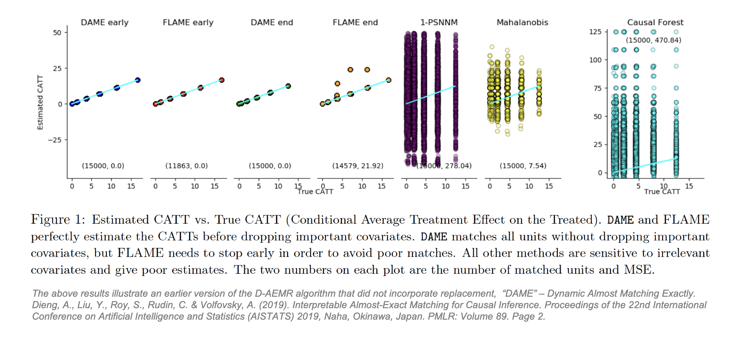
To address PSM’s shortfalls in finding these causal effects, plus the issue that likelihood of finding well-matched pairs decreases in high dimensional covariate spaces, Dieng proposes that observations should still be matched in an n-dimensional space (using a weighted Hamming distance) but only on important covariates. D-AEMR uses machine learning optimization on a hold-out training set to calculate a value of variable importance for each covariate. They define importance as ability to predict the outcome Y, not the ability to predict the probability of being treated, T. The algorithm simultaneously solves all possible optimization problems to identify the “largest (weighted) number of covariates that both a treatment and control unit have in common. [It] fully optimizes the weighted Hamming distance of each treatment unit to the nearest control unit (and vice versa). It is efficient, owing to the use of database programming and bit-vector computations, and does not require an integer programming solver.” [54] D-AEMR also incorporates early stopping to halt the search once the quality of matches starts to decline. Using generated data to estimate a known CATT, they show their algorithm outperforms PSM, MDM and Causal Forest and, unlike the latter, benefits from interpretability. Their code is available on Github [55] but will not be applied here.

PSM with Random Forest
A frequently cited issue with PSM is that misspecification of the propensity score model can lead to poor estimates of the propensity scores and therefore poor matches and biased estimates of the treatment effect. [44] Propensity scores are usually estimated with logistic regression which imposes parametric assumptions relating to the underlying distribution of the population. As matching is a two-step process, these assumptions are compounded when the propensity score is modeled, and the estimation of the treatment effect is modeled. A potential solution to this problem is to approach estimation of the propensity score as any other prediction problem and use state-of-the-art nonparametric machine learning approaches to optimize predictions of the propensity score. [56] Most modeling problems in causal inference deal with unobservable outcomes making highly tuned machine learning algorithms unusable. However, for the propensity score we do observe the outcome of interest. For each individual in the dataset, we directly observe T = 0 or T = 1 and can therefore employ machine learning prediction models to find the best possible propensity scores.

In the coding example below, we will utilize Random Forest and the related Gradient Boosting algorithm estimate the propensity scores. Random Forest, proposed by Breiman, 2001 [57], builds an ensemble of classification trees and uses bootstrapping to combat overfitting. Gradient Boosting is a related algorithm but differs in the order in which the trees are built: where Random Forest builds trees concurrently, Gradient Boosting builds them sequentially, each time correcting the errors of the previous trees. Assuming that a stellar propensity score estimate will translate to an unbiased estimate of the ATT, then these machine learning models should outperform the model where the propensity score is estimated with logistic regression. In the application below, we will estimate the ATT with PSM where the propensity score is estimated by logistic regression and compare it with the estimated ATT from PSM where the propensity score is estimated with Random Forest / Gradient Boosting and cross-validation. For additional details and implementation of this method, see Section 8 below.

5. Outline of Our Methodological Approach for Comparing Matching Methods

In this practical application, we apply five distinct matching methods to pre-process six distinct simulated datasets. The purpose of this application is twofold: 1) To ground the theoretical and statistical assumptions we outlined previously in replicable code, and 2) To compare how well each method estimates the ATT in order to be able to provide some recommendations for using matching methods. As the goal here is to compare matching, the estimation of the ATT (Step 2 of 2) is consistent across all methods, the only distinction is the matching method (Step 1 of 2). Step 2 of 2, estimating the ATT, will be done utilizing the Zelig function native to the MatchIt Package in R. [51]

We will use synthetic data generation, a common approach in machine learning research. By coding the data generating process ourselves, we can control all characteristic attributes of the dataset, and importantly, calculate the true treatment effects. There are ample causal inference publications that use simulated data [58], so we will use their recommendations in setting interesting parameters for our generated data.

6. Evaluation Metrics: Known ATT / Mean Absolute Error

As we will subsample the control group by matching control to treated units and prune non-matched controls, the quantity of interest here is the ATT. The simulated data generates a vector of treatment effects so we can directly calculate the known ATT (the average of the treatment effects across all treated units).

We hope to find at least one method that perfectly estimates the known ATT. It is likely, however, that our estimates will deviate from this true ATT and, as such, we require a metric of error to calculate how far they have deviated. We will compare the known ATT with the estimated ATT of each method using the Mean Absolute Error (MAE). The MAE is a measurement of the absolute difference between two continuous variables. We use the absolute difference as some models may estimate a negative ATT. (As we are comparing just one quantity here (the ATT), the MAE is more simply the Absolute Error between known and estimated ATT.)

7. Synthetic Data Generating Process (DGP) to Generate 6 Datasets

We utilize a DGP package created by our seminar classmates to create our synthetic datasets. Their DGP code is available on GitHub as a Python package “Opossum” [59] and provides excellent parameter settings to generate datasets that closely resemble observational studies. The common attributes and unique parameter settings are outlined here:

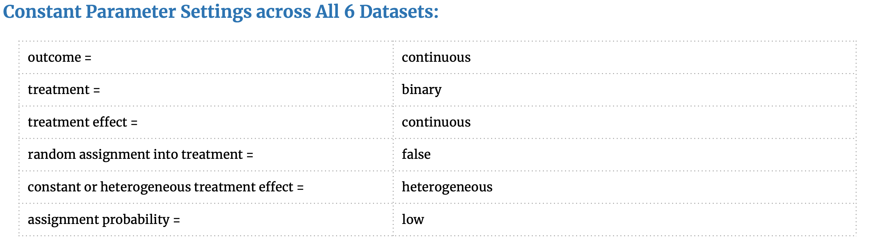
These parameter choices were inspired by our matching research, the available settings in the Opossum package, and helpful recommendations from Dorie (2018) [58] that outlines the simulated DGP from a causal inference competition. Our rationale for choosing these parameter settings is as follows:

• Random assignment into treatment = False, as we are simulating an observational study where the probability of treatment is determined by X.
• Treatment Effect = heterogeneous as would like the treatment effect to vary across different sub-groups of the population as is common in observational studies and produces differing CATT for each sub-group.
• Assignment probability = low as we would like the datasets to have C units » T units. This is common in observational studies: from a large pool of control individuals some are selectively matched to a small treated group. The “low” setting produces a dataset with 35% treated units and 65% control units.
• We create two datasets (small and small_cat*) with low dimensions and observations to determine if any one matching method performs better on low-dimensional data and if any one method performs better with categorical data.
• One dataset (noTreat_k50) with no treatment effect is created in order to see how susceptible the matching methods are to general noise.
• All the datasets feature positive, heterogeneous treatment effects, but the dataset weights_k30 augments this heterogeneity by specifying 60% positive, 20% negative and 20% no treatment effect.
• The final two datasets are inspired by frequent claims in matching literature that matching methods are susceptible to irrelevant covariates. To see if this is true, we create one dataset cond_assign with k=100 but the treatment assignment is determined by only 10 of the covariates and cond_treat with k=100 but the treatment effect is determined by only 10 of the covariates. This concept in causal inference is referred to as “degree of alignment” and is recommended for causal inference DGP [58].

8. Match (and Estimate ATT) with:

1. Coarsened Exact Matching
2. Nearest-Neighbor Propensity Score Matching, with Propensity Score estimated with Logistic Regression
3. Nearest-Neighbor Propensity Score Matching, with Propensity Score estimated with Random Forest
4. Nearest-Neighbor Propensity Score Matching, with Propensity Score estimated with XGBoost
5. Genetic Matching

1. Coarsened Exact Matching

The idea of CEM is to temporarily coarsen each variable into substantively meaningful groups, exact match on these coarsened data and then only retain the original (uncoarsened) values of the matched data.

Algorithm: The CEM algorithm then involves three steps [61] :

1. Temporarily coarsen each control variable in X (covariates) according to user-defined cutpoints, or CEM’s automatic binning algorithm, for the purposes of matching. For example, years of education might be coarsened into grade school, middle school, high school, college, graduate school.
2. Sort all units into strata, each of which has the same values of the coarsened X.
3. Prune from the data set the units in any stratum that do not include at least one treated

[Source:https://medium.com/@devmotivation/cem-coarsened-exact-matching-explained-7f4d64acc5ef]

With every member having a BIN Signature, each is matched to other members with that same BIN Signature. There will likely be an imbalance between the number of Treatment and Control members with a BIN Signature. This variance in distribution must be normalized using CEM Weights.

• All unmatched members get a weight of 0 (zero) and thus are effectively thrown out.
• Matched treatment members get a weight of 1 (one).
• Matched control members get weights above 0 that can be fractional or ≥ 1 that will normalize the BIN signature (archetype) to the distribution within the treatment group.

The formula being:

**Weight = (Treatnment_N / Control_N) / ( Total_Control_N / otal_Treatment_N)**
Now the matched & weighted Treatment and Control members can be compared by using the weights to evaluate the presence & extent of the Treatment Effect.

Problems that can be encountered:

• Matching can be completely off if the wrong variables are chosen.
  Example: There may be dramatic differences between male / female members, if matching does not consider gender, then the matching may never work.
• If the right variables are chosen, but the coarsening is too loose.
  Example: Age could be binned into 1 or 0 depending on if a member is ≥ 50 years old or < 50 years old — for some studies that might be appropriate, but working on a geriatric study, almost everyone will be≥ 50 years old, and this coarsening strategy is inappropriate and too lose.

We can perform CEM matching using MatchIt package in R, by passing the name of the method to MatchIt as “cem” which load the cem package automatically.

  #Perform cem matching to estimate the ATT
  calc_cem <- function(data, psFormula){
    cemMatching <- matchit(psFormula, data = data, method = "cem")
    return(cemMatching)
  }

• psFormula: is the matching fomula “treat ~ covariate1 + covariate2 + …”

Important Note Regarding CEM: if we look a bit below in the section 9 where we show the results of our comparative of matching methods, we will notice there are no results from the CEM Unfortunately. We have encountered an error “subscript out of bounds” while trying to match using CEM MatchIt function in R. After doing some searches, it turns that is a common bug in the MachIt package as mentioned in:
https://lists.gking.harvard.edu/pipermail/matchit/2017-August/000733.html
https://lists.gking.harvard.edu/pipermail/matchit/2009-April/000271.html
https://lists.gking.harvard.edu/pipermail/cem/2013-August/000120.html
And even after we have tried to apply some of the proposed solutions, we kept getting the same error.

2. Nearest-Neighbor Propensity Score Matching, with Propensity Score estimated with Logistic Regression:

Greedy nearest neighbor is a version of the algorithm that works by choosing a treatment group member and then choosing a control group member that is the closest match. It works as follows:

1. Randomly order the treated and untreated individuals
2. Select the first treated individual i and find the untreated individual j with closest propensity score.
3. If matching without replacement, remove j from the pool.
4. Repeat the above process until matches are found for all participants.

There are some important parameter to consider:

• with or without replacement: with replacement an untreated individual can be used more than once as a match, whereas in the latter case it is considered only once.
• one-to-one or one-to-k: in first case each treated is matched to a single control whereas in the latter case each treated is matched to K controls.
• caliper matching: a maximum caliper distance is set for the matches. A caliper distance is the absolute difference in propensity scores for the matches. As a maximum value is being set, this may result in some participants not being matched (Rosembaum and Rubin (1985) [60] suggest a caliper of .25 standard deviations).

In our study we perform a one-to-one greedy nearest neighbor matching with replacement and with caliper to estimate the ATT

# matching on Nearest Neighbor
greedyMatching <- matchit(psFormula, distance = Ps_scores,
                            data = data,
                            method = "nearest", ratio = 1, replace = T, caliper = 0.25)

• distance: are the propensity scores
  
• data: the name of the dataset
• method: nearest neighbor
  
• ratio = 1: one-to-one matching
  
• replace = T: matching with replacement

Disadvantages: Greedy nearest neighbor matching may result in poor quality matches overall. The first few matches might be good matches, and the rest poor matches. This is because one match at a time is optimized, instead of the whole system. An alternative is optimal matching, which takes into account the entire system before making any matches (Rosenbaum, 2002). When there is a lot of competition for controls, greedy matching performs poorly and optimal matching performs well. Which method you use may depend on your goal; greedy matching will create well-matched groups, while optimal matching created well-matched pairs (Stuart, 2010)[4].

In order to perform nearest neighbor matching or any other propensity score based methods, first propensity scores must be estimated. In our study we perform greedy nearest neighbor matching using propensity scores estimated using three different models:

• Logistic Regression
• Random Forest
• Generalized Gradient Boosting

Propensity Score Estimation

The idea with propensity score matching is that we use a logit model to estimate the probability that each observation in our dataset was in the treatment or control group.Then we use the predicted probabilities to prune out dataset such that, for every treated unit, there’s a control unit that can serve as a viable counterfactual.

The estimation of propensity scores could be done using:

• Statistical models: logistic regression, probit regression
  • Mostly widely used
  • Relay on functional form assumption
• Machine learning algorithms: classification trees, boosting, bagging, random forests
  • Do not rely on functional form assumptions
  • It is not clear whether these methods on average better than binomial models

Logistic Regression:

Logistic regression of treatment Z on observed predictors X

• logit(Z_i = 1 | X) = $B$₀ + $B$₁X_1i + …$B$_kX_ki
• Estimated PS:
  • e_i(X) = exp(logit(Z_i = 1 | X)) / 1 + exp(logit(Z_i = 1 | X))

In R we get the propensity scores using logistic regression by calling glm() function, then we calculate the logit of the scores in order to match on, because it is advantageous to to match on the linear propensity score (i.e., the logit of the propensity score) rather than the propensity score itself, bacause it avoids compression around zero and one.

  lr_ps <- function(dataset, psFormula){
      #estimate propensity scores with logistic regression
      lr <- glm(psFormula, data = dataset, family=binomial())

      # It is advantageous to to match on the linear propensity score (i.e., the logit of the propensity score)
      rather than the propensity score itself, bacause it avoids compression around zero and one.
      # log(e(X)) = log(e(X) / 1-e(X))
      lr_estimations <- log(fitted(lr)/(1-fitted(lr)))
      return(lr_estimations)
  }

3. Nearest-Neighbor Propensity Score Matching, with Propensity Score estimated with Random Forest

Random forest, like its name implies, consists of a large number of individual decision trees that operate as an ensemble. Each individual tree in the random forest spits out a class prediction and the class with the most votes becomes our model’s prediction.

The fundamental concept behind random forest is a simple but powerful one — the wisdom of crowds.

A large number of relatively uncorrelated models (trees) operating as a committee will outperform any of the individual constituent models.

The low correlation between models is the key. Uncorrelated models can produce ensemble predictions that are more accurate than any of the individual predictions. The reason for this wonderful effect is that the trees protect each other from their individual errors (as long as they don’t constantly all err in the same direction). While some trees may be wrong, many other trees will be right, so as a group the trees are able to move in the correct direction.

We estimate the propensity score using random forest with the R package party using the function cforest().

rf_ps <- function(dataset, psFormula){
    #estimate propensity scores with random forests
    mycontrols <- cforest_unbiased(ntree=10000, mtry=5)
    mycforest <- cforest(psFormula, data=dataset, controls=mycontrols)

    #obtain a list of predicted probabilities
    predictedProbabilities <- predict(mycforest, type="prob")

    #organize the list into a matrix with two columns for the probability of being in treated and control groups.
    #keep only the second column, which are the propensity scores.
    pScores <- matrix(unlist(predictedProbabilities),,2,byrow=T)[,2]

    #convert propensity scores to logit
    rf_estimations <- log(pScores/(1-pScores))
    return(rf_estimations)
}

• ntree: Number of trees to grow for the forest.
• mtry: number of input variables randomly sampled as candidates at each node

4. Nearest-Neighbor Propensity Score Matching, with Propensity Score estimated with XGBoost

• Boosting is a general method to improve a predictor by reducing prediction error.This technique employs the logic in which the subsequent predictors learn from the mistakes of the previous predictors. Therefore, the observations have an unequal probability of appearing in subsequent models and ones with the highest error appear most. (So the observations are not chosen based on the bootstrap process, but based on the error).
• GNB for propensity score estimation improves prediction of the logit of treatment assignment:
  
  • logit(Z_i = 1 | X)
• Starting value:
  • log[$\bar{Z}$ / (1 - $\bar{Z}$)]
• Regression trees are used to minimize the within-node sum of squared residual:
  • Z_i - e_i(X)
    

Stopping GMB: There is no defined stopping criterion, so errors decline up to a point and then increase, for propensity score estimation, McCaffrey [62] recommended using a measure of covariate balance, to stop the GMB algorithm the first time that a minimum covariate balance is achieved, but there is no guarantee that better covariate balance would not be achieved if the algorithm runs additional iteration.

We use the twang package in R [63] to produce propensity score estimation using GMB, which contains a set of functions and procedures to support causal modeling of observational data through the estimation and evaluation of propensity scores and associated weights. The main workhorse of twang is the ps() function which implements generalized boosted regression modeling to estimate the propensity scores.

# library for ps() function
library(twang)

#Estimate propensity scores with generalized boosted modeling (GBM)
gbm_ps <- function(dataset, psFormula){
  # es: refers to standardized ef-fect size.
  myGBM <- ps(psFormula, data = dataset, n.trees=10000, interaction.depth=4,
              shrinkage=0.01, stop.method=c("es.max"), estimand = "ATT",
              verbose=TRUE)

  #extract estimated propensity scores from object
  gbm_estimations <- myGBM$ps[, 1]
  return(gbm_estimations)
}

• n.trees: is the maximum number of iterations that gbm will run.
• interaction.depth: controls the level of interactions allowed in the GBM.
• shrinkage: helps to enhance the smoothness of resulting model. The shrinkage argument controls the amount of shrinkage. Small values such as 0.005 or 0.001 yield smooth fits but require greater values of n.trees to achieve adequate fits. Computational time increases inversely with shrinkage argument.
• stop.method: A method or methods of measuring and summarizing balance across pretreat-ment variables. Current options are ks.mean, ks.max, es.mean, and es.max. ks refers to the Kolmogorov-Smirnov statistic and es refers to standardized ef-fect size. These are summarized across the pretreatment variables by either the maximum (.max) or the mean (.mean).

5. Genetic Matching

Genetic Matching Offers the benefit of combining the merits of traditional PSM and Mahalanobis Distance Matching (MDM) and the benefit of automatically checking balance and searching for best solutions, via software computational support and machine learning algorithms. Genetic Matching matches by minimizing a generalized version of Mahalanobis distance (GMD), which has the additional weight parameter W . Formally

Genetic Matching matches samples on their weighted Mahalanobis distances calculated from the distance matrix including propensity scores and other functions of the original covariates.

GM adopts an iterative approach of automatically checking and improving covariate balance measured by univariate paired t-tests or univariate Kolmogorov-Smirnov (KS) tests. In every iteration, weights used in the distance calculation are adjusted to eliminate significant results from the univariate balance tests from the end of the last iteration.

The iterative process ends when all univariate balance tests yield non-significant results. GM loosens the requirement on ellipsoidal distribution of covariates.

Below the Flowchart describes how the Genetic Matching algorithm works [13]:

In order to perform Genetic matching, we have to make the following decisions:

1. what variables to match on
2. how to measure post-matching covariate balance
3. how exactly to perform the matching.

Genetic Matching may or may not decrease the bias in the conditional estimates. However, by construction the algorithm will improve covariate balance, if possible, as measured by the particular loss function chosen to measure balance.

We can perform the genetic matching in R, by calling the MatchIt package, in our study we performed genetic matcing on the covariates and the propensity scores estimated by the generalized boosted model

# perform genetic matching based on all the covariates and the propensity score estimated from GMB
calc_geneticMatchin_with_gmb = function(data, psFormula, Ps_scores){
 geneticMatching <- matchit(psFormula, distance = Ps_scores,
                            data = data, method = "genetic", pop.size = 1000,
                            fit.func = "pvals",
                            estimand = "ATT", replace = T, ties = T, discard = "both")
 return(geneticMatching)
}

• pop.size: the number of individuals genoud uses to solve the optimization problem, i.e. the number of the weight matrixes that will be generated in order to have a perfect balance.
• fit.func: The balance metric genetic matching should optimize, here we have chosen “pvals” and that maximize the p.values from (paired) t-tests and Kolmogorov-Smirnov tests conducted for each column in BalanceMatrix
• estimated = “ATT”: the type of the estimated treatment effect, which here is specified as estimated treatment effect on the treated.
• ties = T: A logical flag for whether ties should be handled deterministically. If, for example, one treated observation matches more than one control observation, the matched dataset will include the multiple matched control observations and the matched data will be weighted to reflect the multiple matches. The sum of the weighted observations will still equal the original number of observations. If ties = FALSE, ties will be randomly broken.
• discarded = “both”: a vector of length n that displays whether the units were ineligible for matching due to common support restrictions. In case discarded = both, then both treatment and control unit that are not in the common support will not be matched on.

After Matching Analysis and Estimating ATT:

There are different ways of estimating ATT. We decide to follow the approach suggested by (Ho, D., Imai, K., King, G. & Stuart) [42] using Zelig [64], Which is an R package that implements a large variety of statistical models (using numerous existing R packages) with a single easy-to-use interface, gives easily interpretable results by simulating quantities of interest, provides numerical and graphical summaries, and is easily extensible to include new methods. We estimate the average treatment effect on the treated in a way that is quite robust. We do this by estimating the coefficients in the control group alone. After conducting matching method on our data we go to Zelig, and in this case choose to fit a linear least squares model to the control group only:

# Estimating ATT
get_estimated_treatment <- function(matching_output, zeFormula){
  z.out <- zelig(zeFormula , data = match.data(matching_output, "control"), model = "ls")
  x.out <- setx(z.out, data = match.data(matching_output, "treat"), cond = TRUE)
  s.out <- sim(z.out, x = x.out)
  return(s.out)
}

We pass the to Zelig the formula which has the form “Outcome_Variable ~ covariate1 + covariate2 + …” and where the “control” option in match.data() extracts only the matched control units and ls species least squares regression. Next, we use the coefficients estimated in this way from the control group, and combine them with the values of the covariates set to the values of the treated units. We do this by choosing conditional prediction (which means use the observed values) in setx(). The sim() command does the imputation. The sim() function returns the predicted and the expected values of the ATT and it’s intervals. We take the expected value of ATT as our estimated ATT because we are studying the effect on the outcome and we not trying to predict the future as suggested by (King, G., Tomz, M., Wittenberg, J.)[65]

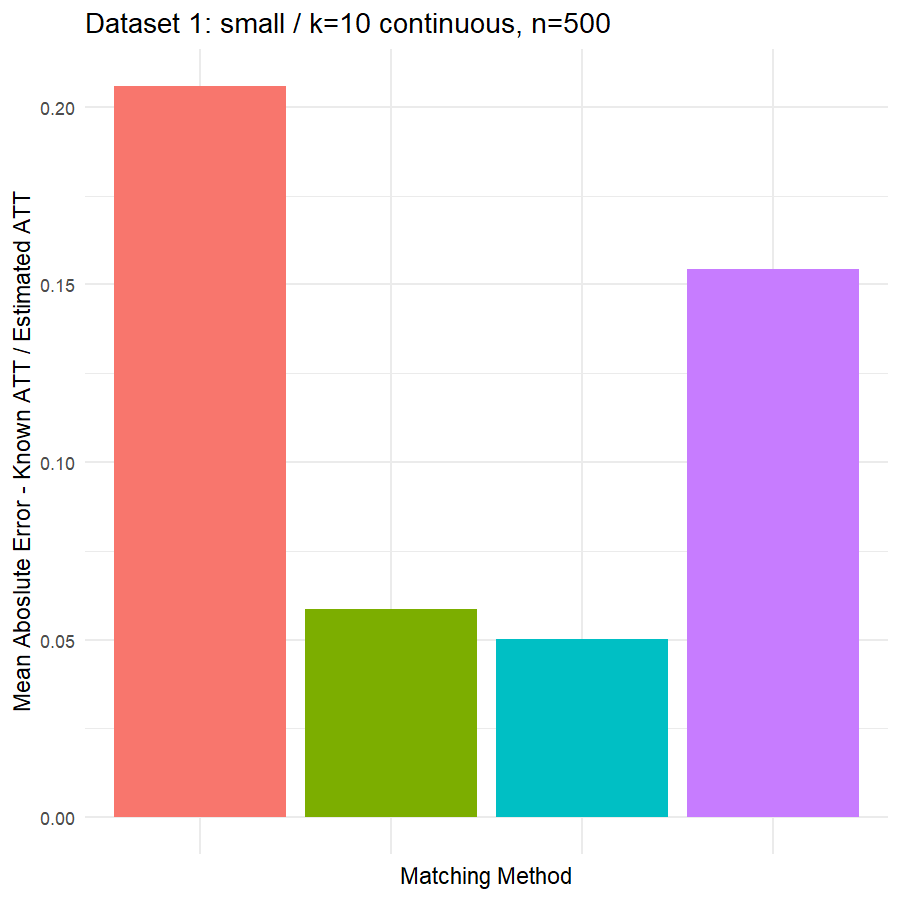
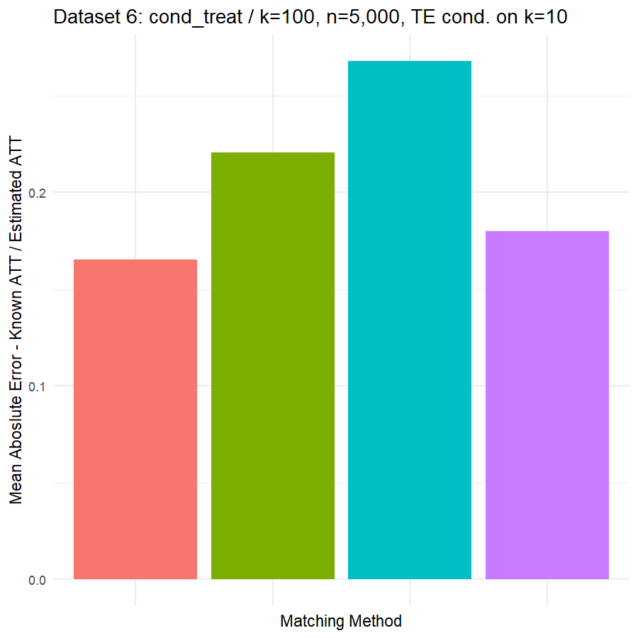
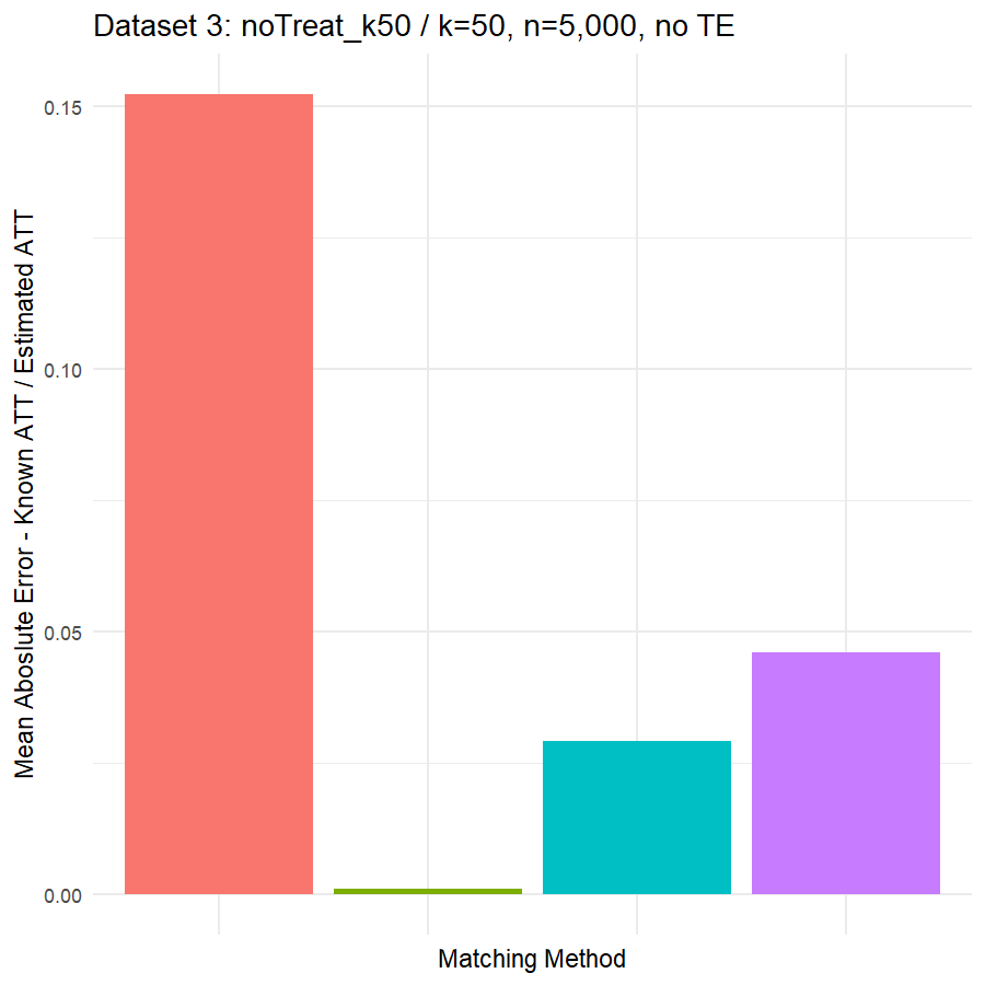
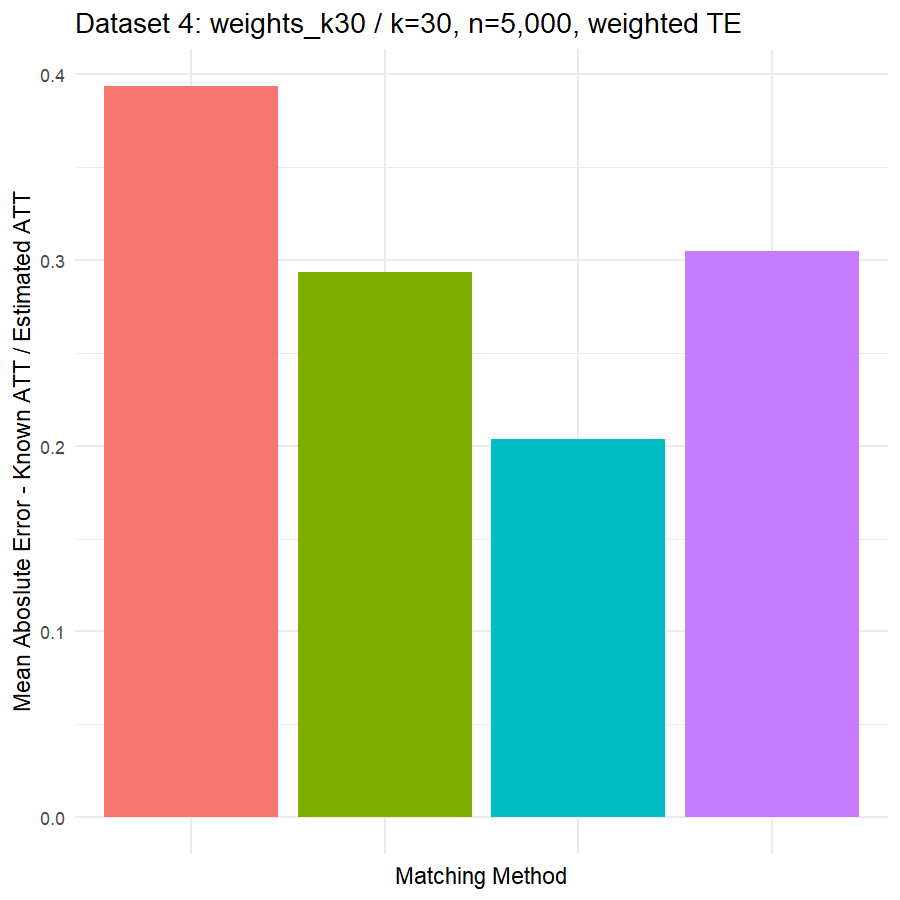
9. Compare Performance of 5 Matching Methods in estimating ATT across 6 Datasets

10. Conclusions & Recommendations: Academic + Results from Our Experiment

We hope that this has been a helpful exploration into the statistical assumptions around matching methods and the recent machine learning developments in the field of matching. The decision to implement matching should come with great care; it is difficult to provide precise recommendations around matching as best practices will vary depending on the dataset at hand. As such, we provide high-level recommendations for researchers considering matching as a preprocessing intervention and point readers to the wealth of literature in the References section for further guidance. In short, the main questions researchers should ask when considering matching is: what is my quantity of interest? Do I care about the group-level estimates, or do I need good individual matches? How much overlap and balance do I have in my data pre-matching? What is the dimensionality of my data? Here are some brief guidelines:

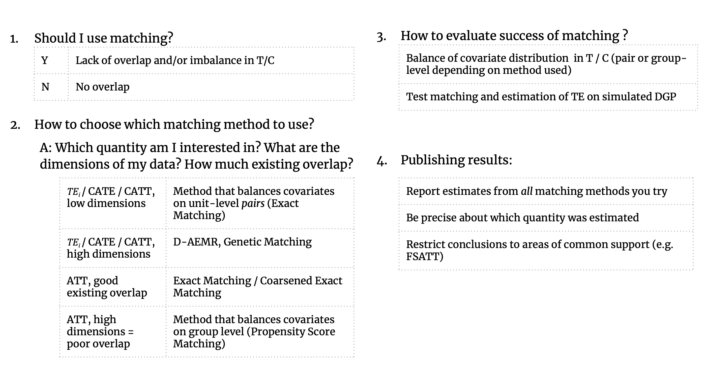
Looking at the results in section 9 from our comparative of matching methods, which they are the mean absolute error in the ATT in five datasets after applying four different matching methods, namely:

• Nearest Neighbor propensity score estimated with Logistic Regression
• Nearest Neighbor propensity score estimated with Random Forest
• Nearest Neighbor propensity score estimated with Generalized Boosting model
• Genetic matching on covariates and propensity score estimated with Generalized Boosting model

We can see clearly, that:

• Genetic matching perform very poorly in all datasets, even it looked to us very attractive theory. Beside the poor results of Genetic matching we have encountered an excessive computational power requirement in order to perform the matching method, especially when the data was highly dimensional.
• Nearest Neighbor with Random Forest and Generalized Boosting propensity score doesn’t perform very bad but also not good as our expectations.
• Our winning model is as always, the simplest model, Nearest Neighbor with Logistic Regression estimated propensity score, we were definitely surprised with its result. In addition of the good results, it was easy to implement and did not required any computational power, beside its possibility of being interpreted, contrary to the other methods which are considered black box models.

11. References

[1] LaLonde, R. (1986). “Evaluating the Econometric Evaluations of Training Programs with Experimental Data.” The American Economic Review, (Vol. 76, No. 4, pp. 604-620). Page 605. Note: The LaLonde study is often invoked as a pedagogical tool in causal inference; the original study included both a randomized trial and an observational study. By estimating the treatment effect from a randomized trial and from observational data ex-post, LaLonde concluded that the econometric techniques in use at the time for estimating treatment effects in observational studies often produced biased estimates.

[2] Guion, R. (2019). Causal Inference in Python. Retrieved 10-08-2019 from: https://rugg2.github.io/Lalonde%20dataset%20-%20Causal%20Inference.html

[3] Angrist, J. & Pischke, J-S. (2008). Mostly Harmless Econometrics: An Empiricist’s Companion. Princeton: Princeton University Press. Page 14.

[4] Stuart, E. (2010). Matching Methods for Causal Inference: A Review and a Look Forward. Statistical Science. Vol. 25, No. 1, 1–21. DOI: 10.1214/09-STS313. Page 1.

[5] Rosenbaum, P., & Rubin, D. (1983). The Central Role of the Propensity Score in Observational Studies for Causal Effects. Biometrika, Vol.70(1), 41-55. Note: This is not the first instance of a matching method used in published statistical research, but Rubin’s proposal for matching on propensity scores propelled the technique into greater esteem in social science research.

[6] Morgan, S. & Winship, C. (2015). Counterfactuals and Causal Inference: Methods and principles for social research. Cambridge: Cambridge University Press. Page 142.

[7] Stuart, 2010. Page 2.

[8] King, G. (2018). Matching Methods for Causal Inference. Published Presentation given at Microsoft Research, Cambridge, MA on 1/19/2018. https://gking.harvard.edu/presentations/matching-methods-causal-inference-3. Slide 5.

[9] There is an interesting discussion between Angrist (of Mostly Harmless Econometrics) and Gelman (of Data Analysis Using Regression and Multilevel/Hierarchical Models) via their blogs around matching. Angrist’s take: http://www.mostlyharmlesseconometrics.com/2011/07/regression-what/ and Gelman’s take: https://statmodeling.stat.columbia.edu/2011/07/10/matching_and_re/

[10] Gelman, A. (2014). Statistical Modeling, Causal Inference and Social Science Blog Post: “It’s not matching or regression, it’s matching and regression.” Retrieved 10-08-2019 from: https://statmodeling.stat.columbia.edu/2014/06/22/matching-regression-matching-regression/

[11] Morgan, 2015. Page 158.

[12] Stuart, 2010. Page 5.

[13] Diamond, A. & Sekhon, J. (2012) Genetic Matching for Estimating Causal Effects: A General Multivariate Matching Method for Achieving Balance in Observational Studies. MIT Press Journals. Review of Economics and Statistics. DOI: 0.1162/REST_a_00318. Page 1.

[14] Stuart, 2010. Page 12. / Graph displays data from: Stuart, E. & Green, K. M. (2008). Using full matching to estimate causal effects in non-experimental studies: Examining the relationship between adolescent marijuana use and adult outcomes. Developmental Psychology 44 395–406.

[15] King, G., Nielsen, R. Coberley, C., Pope, J. & Wells, A. (2011) Comparative Effectiveness of Matching Methods for Causal Inference. Retrieved 10-08-2019 from: https://gking.harvard.edu/publications/comparative-effectiveness-matching-methods-causal-inference. Page 3.

[16] Rubin, D. B. (1974). Estimating Causal Effects of Treatments in Randomized and Nonrandomized Studies. Journal of Educational Psychology, 66(5), 688-701.

[17] King, 2011 (Comparative Effectiveness). Page 2.

[18] Xie. Y., Brand, J., & Jann, B. (2012). Estimating Heterogeneous Treatment Effects with Observational Data. Sociol Methodol. Vol. 42(1): 314–347. Page 3.

[19] King, G., Lucas, C. & Nielsen, R. (2015). The Balance-Sample Size Frontier in Matching Methods for Causal Inference. American Journal of Political Science. Vol.21(2), 473-489. DOI: 10.1111/ajps.12272. Page 6.

[20] Dieng, A., Liu, Y., Roy, S., Rudin, C. & Volfovsky, A. (2019). Interpretable Almost-Exact Matching for Causal Inference. Proceedings of the 22nd International Conference on Artificial Intelligence and Statistics (AISTATS) 2019, Naha, Okinawa, Japan. PMLR: Volume 89. Page 2.

[21] Lam, Patrick. (2017). Causal Inference. Retrieved 10-08-2018 from: http://patricklam.org/teaching/causal_print.pdf ppt

[22] Gelman, A. & Hill, J. (2007). Data Analysis Using Regression and Multilevel/Hierarchical Models. Cambridge: Cambridge University Press. Page 183

[23] Gelman, 2007. Page 184.

[24] Gelman, 2007. Page 183.

[25] Gelman, 2007. Page 199.

[26] Gelman, 2007. Page 201.

[27] Lam, 2017. Slide 12.

[28] Ho, D., Imai, K., King, G., & Stuart, E. (2007). Matching as Nonparametric Preprocessing for Reducing Model Dependence in Parametric Causal Inference. Political Analysis, 15(3), 199-236. DOI:10.1093/pan/mpl013. Page 200.

[29] King, 2015 (Balance-Sample Size Frontier). Page 5.

[30] Dorie, V., Hill, J., Shalit, U., Scott, M., Cervone, D. (2018). Automated versus Do-It-Yourself Methods for Causal Inference: Lessons Learned from a Data Analysis Competition. Statistical Science. Vol. 34(1), 43-68. DOI:10.1214/18-STS667. Page 6.

[31] Sekhon, J. (2008). The Neyman-Rubin Model of Causal Inference and Estimation via Matching Methods. The Oxford Handbook of Political Methodology. DOI: 10.1093/oxfordhb/9780199286546.003.0011. Page 8.

[32] Rosenbaum, P.R. (2005). Heterogeneity and Causality: Unit Heterogeneity and Design Sensitivity in Observational Studies. The American Statistician. Vol59: 147–152.

[33] Morgan, 2015. Page 143.

[34] King, 2011 (Comparative Effectiveness). Page 4.

[35] Iacus, S., King, G. & Porro, P. (2009). Multivariate Matching Methods That Are Monotonic Imbalance Bounding. UNIMI - Research Papers in Economics, Business, and Statistics, Universitá degli Studi di Milano. Retrieved 10-08-2019 from: http://gking.harvard.edu/files/gking/files/cem_jasa.pdf. Page 349.

[36] King, G., & Nielsen, R. (2019). Why Propensity Scores Should Not Be Used for Matching. Political Analysis, 1-20. DOI:10.1017/pan.2019.11. Page 16.

[37] Stuart, 2010. Page 4.

[38] Sekhon, J. (2011). Multivariate and Propensity Score Matching Software with Automated Balance Optimization: The Matching package for R. Journal of Statistical Software. Vol. 42(11). DOI: 10.18637/jss.v042.i07. Page 2.

[39] Stuart, 2010. Page 6.

[40] Aggarwal, C., Hinneburg, A. & Keim, D. (2001). On the Surprising Behavior of Distance Metrics in High Dimensional Spaces. Van den Bussche J., Vianu V. (eds) Database Theory — ICDT 2001. ICDT 2001. Lecture Notes in Computer Science, vol 1973. Springer, Berlin, Heidelberg. DOI: 10.1007/3-540-44503-X_27

[41] King, 2018 (Matching Methods for Causal Inference). Page 2.

[42] Ho, D., Imai, K., King, G. & Stuart, E. (2011). MatchIt: Nonparametric Preprocessing for Parametric Causal Inference. Journal of Statistical Software. Vol 42(2011). DOI: 10.18637/jss.v042.i08. Page 11.

[43] Gelman, 2007. Page 207.

[44] King, 2019 (Why Propensity Score). Page 11.

[45] Unfortunately, the Matching Frontier package was recently removed from CRAN on 2019-05-19; check back for possible updates. The archived version is available at https://cran.rproject.org/src/contrib/Archive/MatchingFrontier/

[46] King, G., Lucas, C. & Nielsen, R. (n.d.) MatchingFrontier: Automated Matching for Causal Inference. Retrieved 10-08-2019 from: https://rdrr.io/cran/MatchingFrontier/f/inst/doc/Using_MatchingFrontier.pdf

[47] King, 2015 (Balance-Sample Size Frontier). Page 13.

[48] King, 2015 (Balance-Sample Size Frontier). Page 24. / Citing: Athey, Susan and Guido Imbens. 2015. A Measure of Robustness to Misspecification. American Economic Review Papers and Proceedings.

[49] King, 2015 (Balance-Sample Size Frontier). Page 1.

[50] Diamond, 2012. Pages 6-7.

[51] CRAN. Package: Matchit. Retrieved 10-08-2019 from: https://cran.r-project.org/web/packages/MatchIt/index.html

[52] Dieng, A., Liu, Y., Roy, S., Rudin, C. & Volfovsky, A. (2019). Almost-Exact Matching with Replacement for Causal Inference. Submitted to arXiv.org Statistics / Machine Learning on 18-06- 2018 (v1), last revised 8-06-2019 (v6). Retrieved 10-08-2019 from: https://arxiv.org/pdf/1806.06802v6.pdf.

[53] Dieng, 2019 (Interpretable). Page 2.

[54] Dieng, 2019 (Almost-Exact). Page 2.

[55] Almost-Exact-Match Github Page. Retrieved 10-08-2019 from: https://github.com/almostExactMatch/daemr

[56] The application of random forest to propensity score estimation has been proposed on several occasions. A few examples are: Kreif, N. & DiazOrdaz, K. (2019). Machine Learning in Policy Evaluation: New Tools for Causal Inference. Submitted to arXiv.org Statistics / Machine Learning on 01-03-2019 (v1). Retrieved 10-08-2019 from: https://arxiv.org/abs/1903.00402. Page 2.

Using ML for Propensity Scores. (2015). The National Bureau of Economic Research. Retrieved 10-08-2019 from: https://www.nber.org/econometrics_minicourse_2015/NBERcausalpredictionv111_lecture2.pdf

[57] Breiman, L. (2001). Random Forests. Machine Learning. 45 (1): 5–32. DOI:10.1023/A:1010933404324.

[58] Dorie, 2018. Pages 8-11.

[59] Opossum GitHub Page. Retrieved 10-08-2019 from: https://github.com/jgitr/opossum/tree/master

[60] Rosenbaum, PR., Rubin, DB., (1985). Constructing a control group using multivariate matched sampling methods that incorporate the propensity score. The American Statistician. 1985;39(1):33–38.

[61] Iacus, S., King, G. & Porro, P. (2009). CEM: Software for Coarsened Exact Matching. Journal of Statistical Software. Vol 30 Issue 9.

[62] McCaffrey, D.F., Griffin, B.A., Almirall, D., Slaughter, M.E., Ramchand, R., and Burgette, L.F. (2013). “A tutorial on propensity score estimation for multiple treatments using generalized boostedmodels.” Forthcoming atStatistics in Medicine

[63]CRAN. Package: twang. Retrieved 02-07-2017 from: https://cran.r-project.org/web/packages/twang/index.html

[64] CRAN. Package: Zelig. Retrieved 22-04-2019 from: https://cran.r-project.org/web/packages/Zelig/index.html

[65] King, G., Tomz, M., Wittenberg, J. (2000) Making the the most of Statistical Analysis: Improving interpretation and Presentation. American Journal of Political Science. 44 (2): 347-361. http://gking.harvard.edu/files/making.pdf