By Seminar Applied Predictive Modeling (SS19) | August 18, 2019
Efficient Experiments Through Inverse Propensity Score Weighting
By Andrew Tavis McAllister & Justin Engelmann
Table of Contents
- Introduction
- Literature Review
- Description of Process
Process in Code
- Imports and Data Generation
- Classical RCT
- Imabalanced Targeting
- Uplift Modeling and Propensity Score Assignment
- Uplift Score Generation
- Propensity Score Derivation
- Assigning Treatment Based on Propensity Scores
- Probability Scaling
- Scaled Propensity Score Derivation / Procedure for propsensity score scaling
- Assign Treatment based on scaled prop score
- Iterated Trials
Accuracy and Cost Based on Targeting Ratio
- Model Noise vs. ATE and Profit
- Visualizing Bias
- Visualizing Distributional Scaling
- The Effect of Bias and Distributional Noise vs. ATE and Profit
- Model Noise vs. ATE and Profit
Summary and Conclusion
Sources
Introduction
As companies and institutions become more data-driven, there is huge potential to make decisions based on scientific A/B-testing, or randomised controlled trials (RCTs), to better estimate causal effects of interventions. Business are becoming more sophisticated in conducting their tests and are moving beyond merely comparing group means to estimate treatment effects.
Traditional Randomised Controlled Trials (RCTs)
Scientists are usually interested in obtaining an accurate and unbiased estimate of the treatment effect. To avoid bias, it is essential that individuals are assigned to the treatment and controls groups at random. To increase accuracy, a natural choice is to assign 50% of the population to the control group and 50% to the treatment group. Thanks to the law of large numbers, more individuals in a group means that the mean treatment effect becomes more accurate, and having splitting individuals evenly means that our estimate is more accurate.
Imbalanced Targeting (IMB)
However, as our overall population increases in size, we can afford to split unevenly to satisfy other objectives. For instance, if we are certain that a treatment will be effective (for instance because we just spent a lot of money on a newly designed website) then we might want to assign more of our population to the treatment group (being shown the new rather than the old website). If, on the other hand, treatment is very expensive, then we might want to assign only a fraction of our population to the treatment group. Suppose that a company is testing a new marketing channel and are currently using a plan with a high cost per customer targeted but no fixed cost. They want to evaluate whether it is worthwhile to switch to a plan with a high fixed cost and no variable cost, so that they could target their entire customer base at no additional cost. To do that, they would need to understand how much of a gain on average by targeting one of their customers, but since at the moment they pay per customer targeted, they'd want to target as few as possible.
In such a scenario, Imbalanced Targeting (IMB) is a good choice. Individuals are still randomly assigned to either group, but instead of splitting them evenly, one of the groups gets assigned more individuals. As long as the smaller group still has sufficiently many members and the assignment is done randomly, a company can still obtain an accurate and unbiased estimate of the treatment effect while satisfying other objectives - such as keeping treatment costs low as in our example. Imbalanced targeting with different proportions of population treated will be our main benchmark.
Propensity Score Weighting
However, while it is an improvement over an RCT, it is still assigning people completely at random. Often, we have at least some idea of who will benefit from treatment more. For instance, suppose that same company has just redesigned their website to make it more appealing to people in general, but to millennials in particular. They think the website is now better at converting any customer (so the treatment effect is always positive), and further plan to switch to it completely. However, normal practice dictates doing an A/B-test with the old website (control) first, to make sure that it is indeed better and to evaluate whether the new website was a worthwhile investment. Thus, they are interested in the average treatment effect (ATE) per visitor, which can then be used to evaluate the monthly benefit of the new website and figure out how long it will be until it paid for itself.
In this scenario, the data practitioner would want to assign more people to the treatment group as, they would expect a strictly positive treatment effect. But assigning more millennials to the treatment group would further be seen as beneficial, as the assumption would be that their treatment effect is especially large. Normally, this is not a good idea as it would introduce selection bias.
Luckily for us, selection bias is a big problem for observational studies, and econometricians and statisticians have come up with clever ways of dealing with it. For instance, if we want to investigate the effect of a voluntary job training program, we have to deal with self-selection bias: people that opt into such a program might be more eager to find a job and more hard-working that the average job seeker. If we compare the average outcome of people that have attended the training program with those that have not, then the difference in mean outcomes is not just caused by the program but also by the selection bias.
To deal with this, we can use inverse propensity score weighting. The idea is that while there is self-selection bias, there is also some randomness involved. Some people that would be likely to attend the program by chance happen to not attend it after all, and vice versa. By weighting each individual by the inverse of their propensity to be in their particular group, we lessen the effect of selection bias.
Propensity Score Targeting (PST)
Normally, someone’s propensity of being in a particular group is unobservable and we have to use heavy statistical machinery to estimate propensity scores. But if we are conducting an A/B-test ourselves, we have full control over who is assigned to what group. We still need to keep the assignment random to avoid biasing our results, but we are free to assign individuals different probabilities of being treated as long as we use inverse propensity score weighting to control for this.
This allows us to assign certain people a higher probability of being treated, according to our expectation of their individual treatment effect. Since we assign those probabilities, we do not need to estimate them after the fact. And since we can make treatment probability conditional on estimated treatment effect, we can use our knowledge about who is most likely to benefit from treatment to make our experiment more efficient. We call this technique Propensity Score Targeting (PST).
In this blog post, we will present the approach in more detail and then conduct a simulation study to compare it with traditional imbalanced targeting.
In our case a person with a higher propensity to be treated will be biased towards having a higher chance of treatment than those with a lower propensity, but will not have an absolute chance of further treatment. Additionally, those with a low propensity will allways have a non-zero chance of treatment. This provides a practical balance between cost maximization based on targeting those that are most likely to respond positively to treatment, as well as adequate data collection on the low propensity group to allow for continued insights into treatment effectiveness. Explained with a simple example, if customers within a certain age range are selected in trials and have a higher propensity to be treated due to higher potential profits, then members of this group would more likely - but not definitely - receive further treatment, and members of other age groups would still always have at least a slight chance of being treated. In this way a practitioner maintains information on the treatment effects on all classes while maximizing the effect of the test at hand. The specific question of our research looks to derive and exemplify the give and take between realized profit and information.
The post proceeds as follows: Section 1 provides an overview of select studies to explain the concepts and advancements in randomized control trials, uplift models, multi-armed bandit problems, and propensity scores - the basis of our experiment; Section 2 presents our experimentation process with steps being justified via the literature; Section 3 shows the process in code; Section 4 presents our results; Section 5 looks into the the result validity given model free parameters; and Section 6 summarizes and concludes.
Literature Review
1.1: $\>$ In the implementation of a randomized control trial, the goal of a researcher or practitioner is primarily to maximize the statistical power of the experiment, minimize the selection bias of groups, and finally to minimize confounding or allocation bias whereby covariates that would effect the trial's outcome are not evenly distributed between treatment and testing groups (Lachin, 1988). To achieve these goals, researchers employ a variety of randomization techniques such as fully randomized assignment, which has issues of sample imbalance; blocked randomization where group sizes are pre-specified (potentially at the covariate level through stratification and random assignment from subgroups), which suffers from selection bias; and adaptive randomization techniques that assign groups based on participant characteristics (Lachin, et. al., 1988). As this project focuses on adaptive techniques, further explication thus follows.
Adaptive randomization procedures can be categorized roughly into covariate-adaptive and response-adaptive techniques. Covariate-adaptive trials attempt to correct for allocation bias via imbalance calculation and correction within the total sample. Response-adaptive trials rather take the prior responses of participants within the testing group as factors for further assignment, attempting to assign groups such that the favorable responses will be elicited (Rosenberger & Lachin, 1988). We will present a response-adaptive style method that will use scaled uplift modeled propensity to assign treatment, thus accounting for prior responses, but again not doing so absolutely.
1.2: $\>$ Uplift modeling attempts to directly model a treatment's incremental impact on the behavior of individual participants, often in cases of imbalanced data. Uplift applied to traditional AB testing with randomized training data allows for the average treatment effect to be analyzed in relation to base demographic information on participants.
Within the practical literature on uplift models, customer classes have been defined via a segmentation of population average treatment effects such that practitioners are aware of target groups and strategies to reach them effectively. Target customers have been broken down into the following groups based on their likelihood to respond to targeting and projected response:
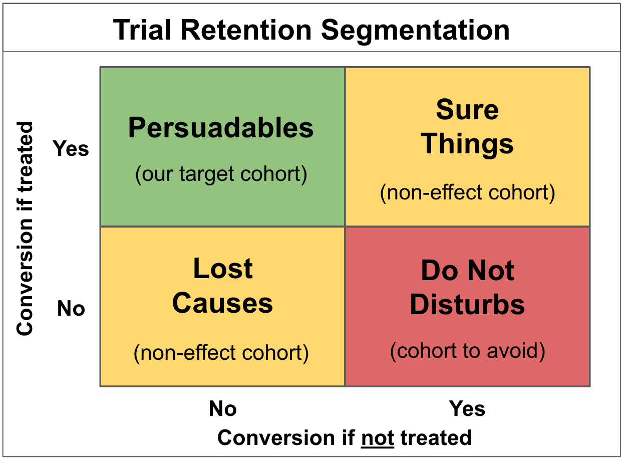
The above displays distinctly that the goal of campaigns is to target "persuadable individuals," avoid "do not disturbs" who would be at risk of churning if targeted, and further reduce any costs associated with treatment with the remaining two groups, as behavior will not be affected. Customer segmentation via uplift modeling thus provides a means to overcome issues with traditional response modeling where in the best scenarios both persuadable individuals and those sure to purchase regardless would be targeted.
1.3: $\>$ Within the context of a catalog mailing we are also presented with a multi-armed bandit problem, which is so named for its modeling of the behavior of slot machine "one armed bandit" strategies. Within such a problem, a practitioner is presented with options to which fixed resources must be allocated, and is thereby tasked with maximizing the profit of the situation at hand (Auer, 2002). Specifically, the practitioner will not fully know the effect of allocation until the simulation or real life experiment has been run, and thus will not know a proper method of exploitation until sufficient exploration of the options has occurred (Weber, 1992). Multi-armed bandit problems can be thought of as examples of Markov decision processes, where the state of the process within which the agent must make decisions would be consistent in examples where no effect on return probabilities is made based on other decisions (a slot machine choice not effecting the probability of another), or would be dependent in examples such as ours where mailings to "do not disturbs" or "persuadables" would negatively or positively effect the margins of a later trial respectively (Vermorel & Mohri, 2005).
Solutions to multi armed bandit problems have evolved in recent years to allow for adaptive behavior through agent learning, and thus are more applicable to a practical setting where the true optimal solution would be unknown, or further would change based on market shifts or technological change (Tokic, 2010; Bouneffouf, et al, 2012). Similarly, bandit problems have also been expanded to include contextual vectors for the given options, which along with prior information can be used by the participant to make more informed decisions (Langford & Zhang, 2008).
1.4:
$\>$ Propensity scores are used to solve the problem of selection bias, where a difference in outcome may be caused by a factor that predicts treatment, rather than the treatment itself, thus implying that a difference in means would not be a true estimator of the ATE. Examples of elements of a score include a participant's natural inclination to be treated, self selection bias, inconsistent use of treatment on the part of researchers, or missing not at random data (Schnabel, et al., 2016). Given a covariate space of characteristics $X$ and a treatment $T$, the scalar propensity score for an individual $i$ is defined by:
Propensity scores are typically estimated with logit models, as normal linear models would produce values for treatment outside of a 0-1 binary, with generalized boosting models becoming more and more popular due to their ability to overcome the often complex functional forms relating propensities (Lambert, 2014; McCaffrey, et al, 2004).
Propensity scores arise directly from the conditional independence assumption (the aptly abbreviated CIA), or unconfoundedness assumption as defined by Rubin (1990). It states that the outcomes $Y_0$ and $Y_1$ of an individual $i$ given a test $T = 0 \; or \; 1$ are independent of the trial so long as the covariates of the individual are accounted for:
Propensity scores and unconfoundedness are linked through a corollary to the latter, the Propensity Score Theorem (PST), which generalizes the CIA conditioning on propensoity scores themselves such that:
The CIA's potentially high dimensionality from $x_i$ is thus reduced to the scalar output of the propensity score function of an individual's covariates, allowing for stratification (or in our case weighting) over one dimension, and further allows for the computation of individual treatment effects (ITEs) across treatment groups. The ability to generalize results across treated and non-treated groups is provided by the following:
The above solves the counterfactual of responses for unobserved treatments for given individuals, $\mathbb{E}[Y_{0i}\;|\;T_{i}=1,P(x_i)]$, given that our response is independent of treatment so long as we are conditioning on propensities. This further allows for a generalization to average treatment effects (Lambert, 2104; Angrist & Pischke, 2009).
Propensity score weighting uses the derived propensities of participants directly for further testing. The distribution of the scores can be derived via the individual covariate spaces of participants given their prior response trials in practical cases, and in theoretical cases can be set or derived via known uplift effects on given individuals. We make use of the latter strategy so that we can focus on the results of such a strategy to derive its utility, with practical cases being left for future analysis and the greater research community.
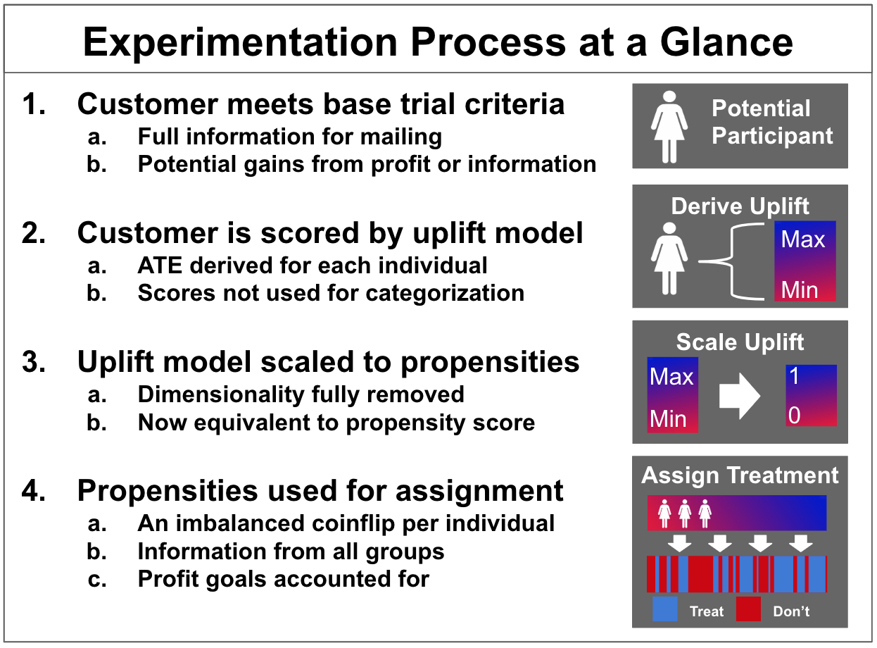
Description of Process
In our process, propensity scores are implemented directly as weights for distributional treatment selection within a catalog mailing campaign. The purpose of this is to provide a practitioner with the ability to gage their degree of interest in the validity of their treatment selections, thus balancing a potential information gain and potential earnings within future trials with a more optimal strategy in the current trial.
The propensity scores of a participant change the chance of treatment and add a pragmatic degree to the trial, whereby the results can be used to inform further decisions. Stated explicitly, explanatory RCTs seek to select participants with highly controlled conditions that give an impression of effectiveness in ideal circumstances, whereas pragmatic trials have relatively unselected participants, allowing for their results to be generalized to normal practices (Zwarentein, et al, 2009). Our technique falls between both methods, providing practitioners with the ability to choose the degree of monetary effectiveness in relation to potential information gain. Within the catalog mailing setting, we further make the hypothesis that the receipt of a catalog will have a positive effect on customer spending (all treatment effects are positive - as seen later in the code), and in that are making a superiority claim about the treatment's effect.
Returning to the multi armed bandit formulation and its eponymous slot machine example, a gambler would not know the best way to exploit the available machines until they have tried them sufficiently. This then relates to our catalog example in that the practitioner would not know proper advertising strategies without first making initial mailings. Spoken of mathematically, the goal of our marketing practitioner is to reduce their regret within dependent Markov states, as the recipients' responses to any given mailing - be they "persuadable," "do not disturbed," etc - will determine the profitability of the next. This is defined as the difference between the practitioner's optimal strategy and that which they have actually earned, but adding further in our case an element of information gain (Vermorel & Mohri, 2005). This further changes the optimal strategy within our setting away from greedy behavior where the highest known return in any round of mailings would be chosen, as such strategies within a practical setting would negate the information gain that would allow for the practitioner to derive a more optimal strategy (it being much less likely in such cases that the practitioner actually knows the true optimal).
The ability of a practitioner within our strategy to balance their information gain and profit goals provides strategies distinct from those normally used within marketing fields. Normally a practitioner would target potential customers via a fully balanced method when the goal is a naive comparison of sample means, but other strategies are also implemented such as an 80-20 target and not-target split, and targeting all individuals over a given threshold of profitability - as was the final suggestion in Hitsch and Misra. In all of these cases, the firm loses information on the class with a low propensity for treatment, and thus loses potentially valuable information on the method's performance (Hitsch, Misra, 2018).
The following diagram depicts our experimental process more explicitly:
Data Simulation and Code
For our simulation study, we assume a catalog setting where the cost of treament is constant throughout our population. We further assume that there is some pre-existing individual uplift model. Individual uplift is just another term for individual treatment effects. Such predicted individual treatment effects could come from a sophisticated causal machine learning approach like Generalized Random Forests, or for a simple expert model ("This treatment works better for older than for younger people".)
For this blog post, we are just interested in (profit-)efficient experiments to estimate the average treatment effect (ATE). That is often enough to make a decision, such as deciding to buy a introduce CRM-system or to switch to a new website. This has a great advantage: to compare our propensity score targeting approach with traditional imbalanced targeting, we just need to simulate two things: The untreated outcome, y_0, and the individual treatment effect. By adding those two up, we contain the treated outcome y_1. Both outcomes and treatment effects have some random variation between individuals.
To simulate having an uplift model, we simply add varying degrees of noise to our simulated treatment effect. As we are not interested in recovering conditional treatment effects here, this is sufficient for our purposes and neatly avoids having to simulate any covariates at all. A deeper simulation with covariates with an actual uplift model is equivalent to just adding random noise to the true treatment effect.
Furthermore, we assume that treatment effects are always larger than treatment cost. This is simply to avoid going down a rabbit-hole of complexity: Given some imperfect individual uplift model and treatment effects that can be both higher or lower than the cost of targeting, we could then try to only treat individuals that have a high chance of being profitable to treat. But this is not the purpose of this simulation, and likely exceeds the complexity of much of the A/B-testing that is done in practice. Alternatively, of course, we culd also assume that treatment effects are always smaller than treatment costs.
Is either of these cases realistic? One could wonder why we would want to estimate the ATE at all, if we know that treatment is always or never a good idea. While the question is very legitimate, there are also many good answers for it. For instance, we might be testing a new marketing measure that is expensive at a small scale, but would be cheaper if we deem it worthwhile. Imagine we are mailing out catalogs for the first time ever: before ordering hundreds of thousands catalogs to send to all of our customers, we might want to do a smaller scale test with only, say, 20,000. Of course, in this case we pay much higher printing and distribution costs for such a small volume than if we ordered hundreds of thousands catalogs instead. Thus, we know that in this case, every catalog we send out will be unprofitable. But what we are interested in is finding out what the average treatment effect is to evaluate whether investing in sending out catalogs to our entire customer base will be profitable.
Many business decisions share this feature: small scale tests often have higher unit costs than large scale implementation. On the other hand, with enterprise software, small scale tests might be completely free (i.e. when testing a new email marketing tool) so that every treatment is profitable in the test, but we are interested in evaluating the average treatment effect to decide whether switching to this software will be worth the annual cost.
We'll now begin explaining the process in code.
Imports and Data Generation
# Basic diagnostics of our simulation
price_of_treatment = 10

# Normal distribution attributes
N = 30000
mean = 50
std = 10
We can assume non-zero costs within our experiment due to tangible catalogs being sent in the style described by Hitsch and Misra. It should also however be noted that data driven email marketing campaigns will potentially not be zero cost endeavors, as campaigns of such size could make use of email marketing services to better organize mailings and the data that they produce, as well as provide base analytics.
We start with an initial response upon which our propensity scores are made. This is generated from the above diagnostics via the combination of a normal and a uniform distribution. The effect of treatment is then generated - again via the combination of a normal and uniform distribution with the mean in this case being 20. Both distributions are pictured below:
y_0 = np.random.normal(loc=3*mean/4, scale=std, size=N) + np.random.uniform((mean/4)-std/4, (mean/4)+std/4, size=N)
y_0 = np.round(y_0, 2)
true_treatment_effect_mean = 20
true_treatment_effect = np.round(np.random.normal(loc=true_treatment_effect_mean,
                                                  scale=1,
                                                  size=N)
                               + np.random.uniform(-true_treatment_effect_mean/5,
                                                   true_treatment_effect_mean/5,
                                                   size=N), 2)
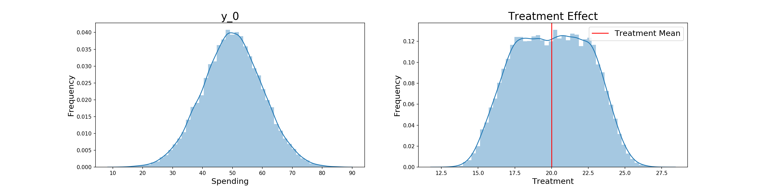
As stated before, the mean and standard deviation of the treatment effect creating a distribution that's always > 10 implies that there is no negative effect of treating an individual.
The initial consumption and treatment effect are then combined to model the customers spending after treatment. Whether they produce this level of spending or that from Y_0 is determined by trial selection, and specifically the weighting criteria to come. The comparison between Y_0 and Y_1 is displayed below.
y_1 = y_0 + true_treatment_effect
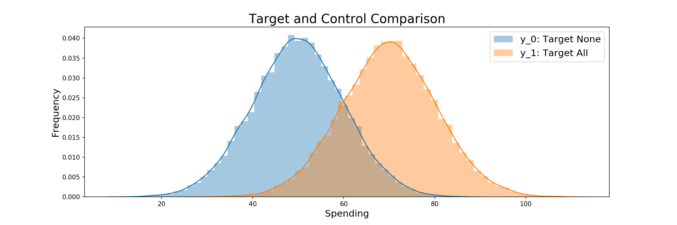
The base profit of the simulation when not targeting anyone or targeting all individuals is then found before RCTs begin. They are as follows:
print('Profit when doing nothing: {}'.format(round(y_0.sum(), 2)))
print('Profit when targeting all: {}'.format(round(y_1.sum() - (price_of_treatment*N))))
Classical RCT
For a first exploration of RCTs, we begin with a classical example where 50% of all individuals are targeted. Randomly generated indexes serve as a mask to derive who will receive their post treatment spending, with profits after treatment being calculated after. The estimated treatment effect is also calculated and compared to the true effect, results showing that the effect was slightly over estimated. Code for the first RCT follows:
def classical_rct():
    """
    Runs a classical RCT with 50% targeting

    Output: spending per customer and a mask of who was targeted
    """
    rct_outcome = y_0.copy() # Initialise outcome with y0
    rct_indices = np.random.choice(a = np.arange(y_0.size),
                                   size = int(y_0.size * 0.5), # 50% target
                                   replace = False)

    rct_outcome[rct_indices] = y_1[rct_indices]
    rct_mask = np.ones_like(y_0, dtype=bool)
    rct_mask[rct_indices] = False

    return rct_outcome, rct_mask
rct_outcome, rct_mask = classical_rct()
Profit from our RCT in comparison with that of the treat none and treat all groups is shown below, falling between that of target none and target all strategies as expected.
The distribution also being plotted in comparison to Y_0 and Y_1.
def print_outcomes(trial_outcome, assignment_mask):
    """
    Prints needed outcomes for each trial given the per customer spending resulting
    from the trial, as well as a mask for who was targeted to derive the EST
    """
    print('Estimated Treatment Effect: {}'.format(round(trial_outcome[~assignment_mask].mean()\
                                                        - trial_outcome[assignment_mask].mean(), 2)))
    print('True Treatment Effect:      {}'.format(round(true_treatment_effect.mean(), 2)))
    print('Profit:         {}'.format(round(trial_outcome.sum(), 2)))
    print('Targeting none: {}'.format(round(y_0.sum(), 2)))
    print('Targeting all:  {}'.format(round(y_1.sum(), 2)))
# Outcomes
print_outcomes(rct_outcome, rct_mask)
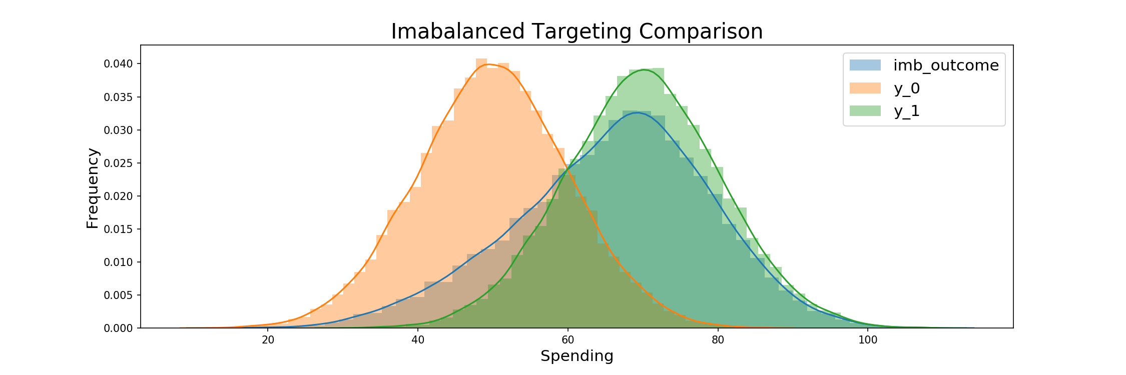
Imabalanced Targeting
Imbalanced targeting is then modeled. The process is the same as before, but in this case treatment assignment being given randomly to 80% of the samples. Profits again fall between that of the target none and target all scenarios as expected, but the high target ratio brings them close to targeting all's profits.
The consumption outcomes and comparison of the resulting distribution to the original Y_0 and Y_1 groups follow:
def imbalanced_targeting(imb_ratio):
    """
    Runs an imbalanced trial with a chosen targeting ratio

    Output: spending per customer and a mask of who was targeted
    """
    imb_outcome = y_0.copy() # Initialise outcome with y0
    imb_indices = np.random.choice(a = np.arange(y_0.size),
                                   size = int(y_0.size * imb_ratio), # Assign imb_ratio
                                   replace = False)

    imb_outcome[imb_indices] = y_1[imb_indices]
    imb_mask = np.ones_like(y_0, dtype=bool)
    imb_mask[imb_indices] = False

    return imb_outcome, imb_mask
imb_outcome, imb_mask = imbalanced_targeting(0.8)
# Outcomes
print_outcomes(imb_outcome, imb_mask)
Uplift Modeling and Propensity Score Assignment
Uplift Score Generation
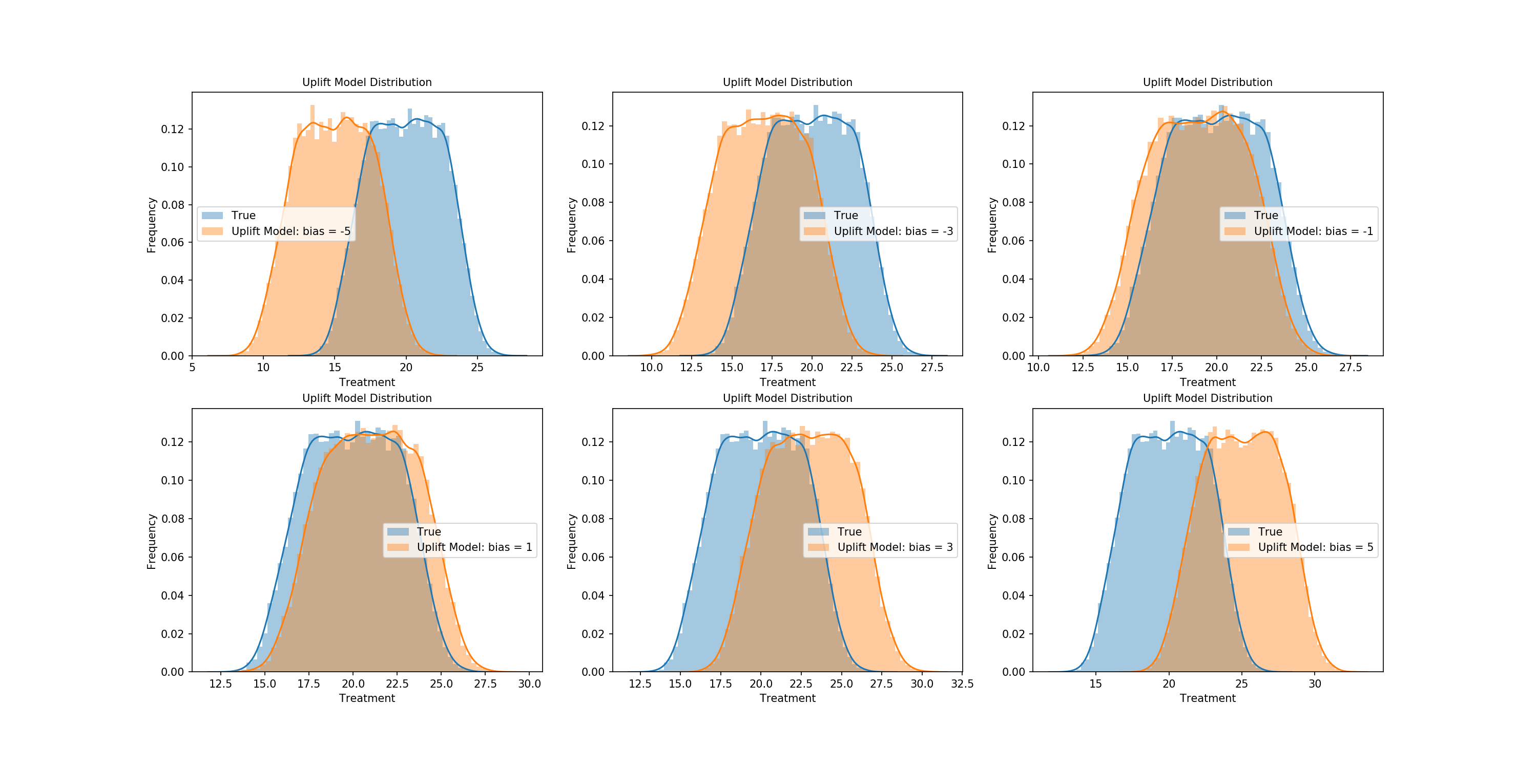
We now begin our method of selection based on propensity score weighting. The true modeling of propensity scores takes the form of a simulated uplift model, which is the true treatment effect with elements of random normal and uniform noise added, as well as a negative bias. The addition of noise adds a degree of robustness to the model to regularize results, which is important given the size of the generated data. Any produced negative values are then replaced with 0. The code to produce the uplift model follows, its comparison to the true treatment effect is graphed, and the relation between true treatment and uplift is also displayed:
def generate_uplift(bias, scale_normal, scale_uniform):
    """
    Generates an uplift score for each customer with inputs being
    the true treatment effect, as well as noise generated from a normal
    distribution and uniform distribution

    Each uplift model has user specified scalers for the normal and
    uniform distribution parameters

    Negative uplift values are mapped to 0
    """
    pred_uplift = np.round(true_treatment_effect
                           + np.random.normal(loc = 0,
                                              scale=true_treatment_effect_mean/scale_normal,
                                              size=N)
                           + np.random.uniform(-true_treatment_effect_mean/scale_uniform,
                                               true_treatment_effect_mean/scale_uniform,
                                               size=N)
                           + bias
                           ,2)

    pred_uplift = np.where(pred_uplift<0, 0, pred_uplift)

    return pred_uplift
pred_uplift = generate_uplift(-2.5, 10, 10)
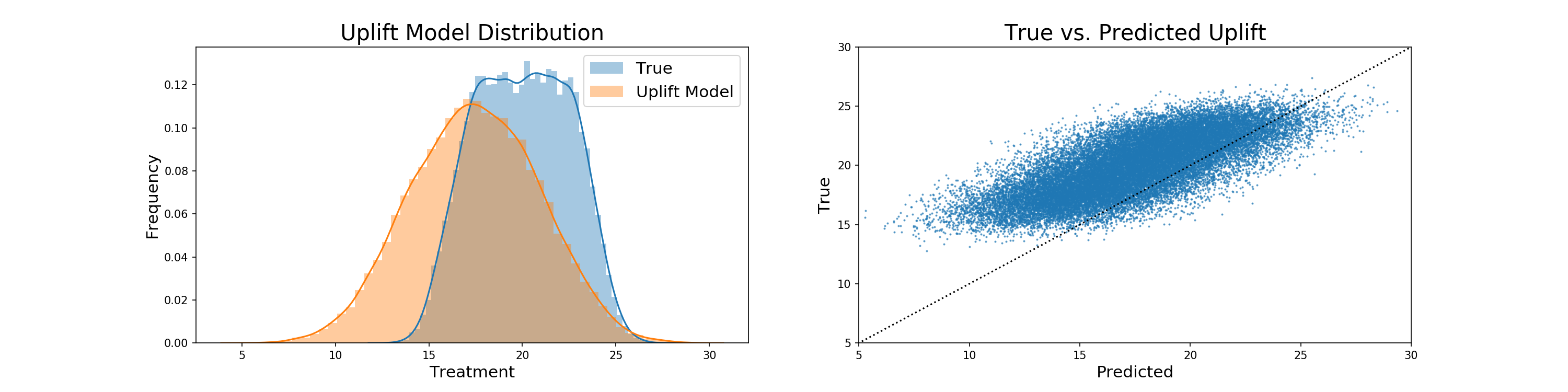
sp.stats.pearsonr(pred_uplift, true_treatment_effect)
pred_uplift.mean()
true_treatment_effect.mean()
We see that the added noise and negative bias means that our uplift model is generally under-predicting the true treatment effect, with the means of the two being 17.5 and roughly 20 respectively.
Propensity Score Derivation
Propensity scores are then derived from the uplift model via scaling. As stated earlier, an uplift model provides us with a per-participant estimate of the average treatment effect. In scaling it, we reduce the range of the already one-dimensional representation of each participants' treatment to that of propensity scores. In this way we do not need covariates to derive the propensity scores, in that we have already calculated the propensity via our hypothetical uplift, and just need the values to be within a 0-1 range to allow for assignment. The code to derive propensities follows:
def assign_prop_scores(uplift):
    """
    Assigns propensity scores via a scaling of predicted uplift values
    """
    assigned_prop_scores = (pred_uplift-pred_uplift.min()+0.01)/(pred_uplift.max()-pred_uplift.min()+0.01)

    return assigned_prop_scores
assigned_prop_scores = assign_prop_scores(pred_uplift)
assigned_prop_scores[:5]
Now that we have our propensity scores, we begin with the tests of our main models. The following code details the use of the scores for an imbalanced 80-20 trial, with the generated scores being the determinants of the final treatment assignment. Assignment follows a similar fashion for each weighting based model.
Assigning Treatment Based on Propensity Scores
def assign_pst_treatment(pst_ratio, prop_scores):
    """
    Assigns customers to treatment via a random choice given their
    personal propensity score
    """
    pst_indices = np.random.choice(np.arange(y_0.size),
                                   size=int(N*pst_ratio),
                                   replace=False,
                                   p=prop_scores/prop_scores.sum())

    pst_outcome = y_0.copy()
    pst_outcome[pst_indices] = y_1[pst_indices]
    pst_mask = np.zeros(y_0.size, dtype=bool)
    pst_mask[pst_indices] = True

    return pst_outcome, pst_mask
pst_outcome, pst_mask = assign_pst_treatment(0.8, assigned_prop_scores)
# Outcomes
print_outcomes(pst_outcome, pst_mask)

Probability Scaling
Scaled Propensity Score Derivation
The following scales the predicted uplifts into a given range. Following the suggestion by Li and Morgan, we choose [0.1, 0.9] to assure that the ATE is not adversely effected by outliers, while at the same time maintaining a diverse distribution. This scaling will be applied to an imbalanced trial before being implemented in the repeated trials.
The goal is to have a distribution centered around a proportion from which we would like to treat. So if we would like to treat 80% of participants, then we want our distribution centered around 0.8, but for the overlying distribution to mimic the outputs of a distribution if it were bounded by the range suggested by Li and Morgen. For the 80% targeting case, this would be a uniform distribution between 0.7 and 0.9.
Procedure for propsensity score scaling
Input: Predicted uplift per customer, desired proportion targeted
Output: Assigned propensity scores per customer
- Sort customers by predicted uplift (ascending) > index each entry [0-n]
- Map indices to desired probability interval
- Divide by n to obtain uniform distribution between 0 and 1 of length 1.
- Multiply by max length of the interval (see formula below) such that our distribution is in the desired interval, [0.1,0.9] - as suggested by Li and Morgan. More extreme scores would lead to individual samples influencing the results too much.
- Add a constant such that we obtain the desired center/mean of the distribution, which is also the expected value (since we have a uniform distribution).
- Return interval.
The maximum length of the interval is given by min( (mean - 0.1) 2 , (0.9 - mean) 2 ), which says that the length of the interval is bounded by either the distance of the mean to the absolute lower bound times two, or the distance to the absolute upper bound times two. We want to use the longest interval we can, as this ensures the highest variation in propensity scores and thus allows us to make the best use of our pre-existing uplift model.
For example, if we want to target 80% of the population, the max length would be min( (0.8 - 0.1) 2, (0.9 - 0.8) 2) = min(1.4, 0.2) = 0.2. So we multiply the uniform distribution, which is currently between [0,1], by 0.2, so that it is between 0 and 0.2. Then we shift the mean to 0.8 as we want to target 80% of the population. The current mean is 0.1, and so we add 0.7. Thus our new distribution is uniform between 0.7 and 0.9 with an expected value of 0.8 – the 80% we desired.
Below, we can see how this mapping is implemented in python code. We can see that our new distribtuion is a) centered at the target ratio and uniform, b) stays in [0.1,0.9] and c) uses the maximum variation given a) and b).
ratio = 0.8
ordered =  sp.stats.rankdata(pred_uplift)-1
ordered = ordered / ordered.size
max_len = min( (ratio - 0.1) * 2 , (0.9 - ratio) * 2 )
ordered = ordered * max_len
assigned_prop_score = ordered + (ratio - ordered.mean())


Assign Treatment based on scaled prop score
scaled_pst_outcome, scaled_pst_mask = assign_pst_treatment(scaled_pst_ratio, scaled_sorted_prop_scores)
# Outcomes
print_outcomes(scaled_pst_outcome, scaled_pst_mask)
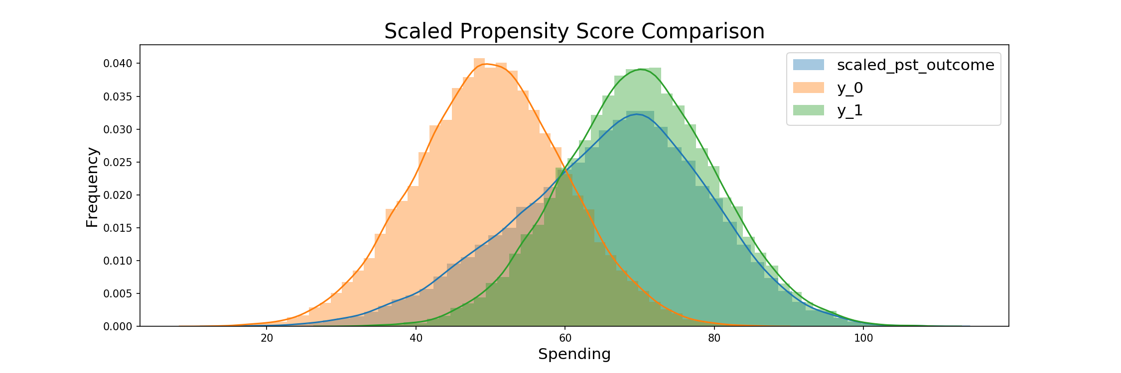
The above strategy has the advantage of being able to scale any distribution of uplift - regardless of how asymmetric it is. The results always being a normal distribution could be seen as problematic, but also have the advantage of counteracting potentially strong localization in model results. A further problematic case of such a strategy is that it is limited to targeting within the scaled distribution, so in our case from 10 - 90%, but this provides a range that's well within the bounds of normal RCT testing.
Iterated Trials
Accuracy and Cost Based on Targeting Ratio
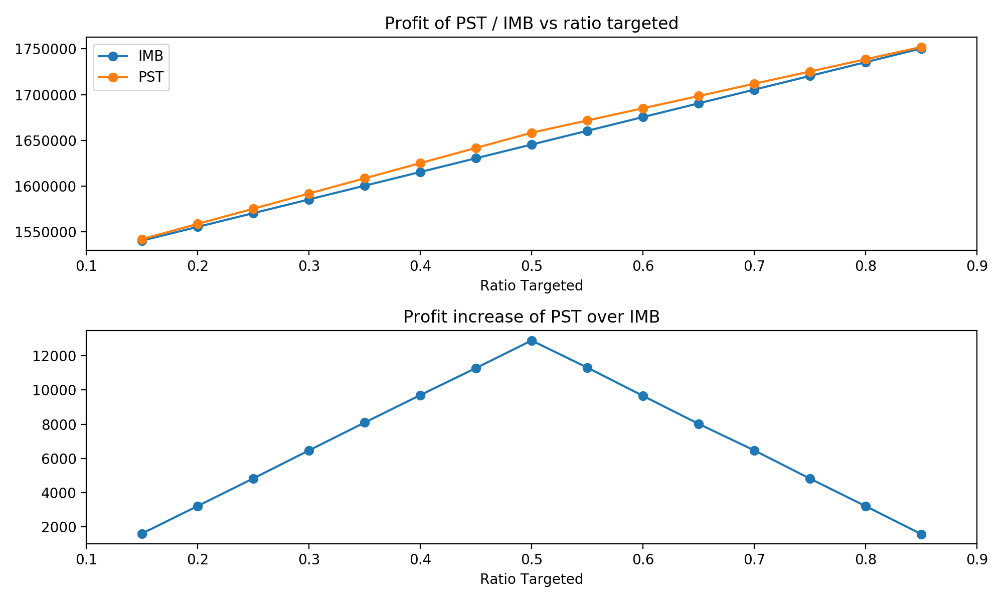
Now it is time for the core of our analysis. We understand how both techniques work, how the data is simulated and what results we are expecting. Now we simulate both approaches for target ratios: from 0.15 to 0.85, going in steps of 0.05. At each ratio, we iterate both approaches 500 times and save the results: ATE, absolute error of the ATE estimate from the true value, and profit increase due to treaments (total treatment effect less total treatment costs).
# Make a data frame to store results
results_df = pd.DataFrame()
sim_iterations = 500
list_of_ratios = np.round(np.arange(0.15, 0.9, 0.05),2)
for ratio in list_of_ratios:
    for i in range(sim_iterations):
        #RCT / IMB
        rct_outcome = y_0.copy() # initialise outcome with y0
        # randomly assign the desired proportion > since all individuals have the same chance to be selected,
        # we can go with simple drawing without replacement
        rct_indices = np.random.choice(a = np.arange(y_0.size),
                                              size = int(y_0.size * ratio), replace = False)
        rct_outcome[rct_indices] = y_1[rct_indices]
        rct_mask = np.ones_like(y_0, dtype=bool)
        rct_mask[rct_indices] = False
        results_df.loc[i,'RCT_ATE_' + str(ratio)] = rct_outcome[~rct_mask].mean() - rct_outcome[rct_mask].mean()
        results_df.loc[i,'RCT_AE_' + str(ratio)] = np.abs((rct_outcome[~rct_mask].mean() - rct_outcome[rct_mask].mean())
                                                          - true_treatment_effect_mean)
        results_df.loc[i,'RCT_PI_' + str(ratio)] = rct_outcome.sum()-(ratio*N*price_of_treatment)

        #PST
        # here we use true random assignment
        # scaling propensity scores: (as above)
        ordered =  sp.stats.rankdata(pred_uplift)-1
        ordered = ordered / ordered.size
        max_len = min( (ratio - 0.1) * 2 , (0.9 - ratio) * 2 )
        ordered = ordered * max_len
        assigned_prop_scores = ordered + (ratio - ordered.mean())
        pst_mask = np.array([random.random()<=prob for prob in assigned_prop_scores])
        # weights for targeted / non-targeted -  inverse propensity score weighting
        weights_targeted = np.array([1/p for p in assigned_prop_scores[pst_mask]])
        weights_not_targeted = np.array([1/p for p in assigned_prop_scores[~pst_mask]])

        pst_outcome = y_0.copy()
        pst_outcome[pst_mask] = y_1[pst_mask].copy()
        results_df.loc[i,'PST_PI_' + str(ratio)] = pst_outcome.sum()-(pst_mask.mean()*N*price_of_treatment)
        pst_outcome[~pst_mask] = pst_outcome[~pst_mask] * weights_not_targeted
        pst_outcome[pst_mask] = pst_outcome[pst_mask] * weights_targeted
        results_df.loc[i,'PST_ATE_'+ str(ratio)] = ((pst_outcome[pst_mask].mean()/weights_targeted.mean())
                                           - pst_outcome[~pst_mask].mean()/weights_not_targeted.mean())
        results_df.loc[i,'PST_AE_' + str(ratio)] = np.abs((((pst_outcome[pst_mask].mean()/weights_targeted.mean())
                                           - pst_outcome[~pst_mask].mean()/weights_not_targeted.mean())
                                                          - true_treatment_effect_mean))

        if i+1 == sim_iterations:
            print('Done with iteration {} / {} for ratio {}'.format(i+1, sim_iterations, ratio))
Here are the results for a first look, detailed interpretation follows in the conclusion.
Model Noise vs. ATE and Profit
The following details the effect of noise within our uplift model on the average treatment effect and profits. This will help us better derive what the effect of a potentially more or less noisy model might have, thus giving us a better understanding of result robustness. As a reminder, within the iterated trials we set:
- Uplift bias to -1
- Uplift normal scaling to 50
- Uplift uniform scaling to 50
Visualizing Bias
Let's start by graphically representing the effects of certain free uplift parameters. The effects of bias are first plotted, with negative and positive values of varying degrees being shown so we can better understand its effect on scaling the true treatment effect.
bias_uplift_dict = {}
possible_biases = [-5,-3,-1,1,3,5]

for bias in possible_biases:
    pred_uplift = generate_uplift(bias, 50, 50)
    bias_uplift_dict[str(bias)] = pred_uplift
Visualizing Distributional Scaling
Next we'll look at the effects of the scalers used on the true treatment effect within the production of the uplift model. Let's first graph the normal and uniform components of our uplift model so we have a general intuition of its construction.
# Same as in the iterated trials
normal_componenet = np.random.normal(loc = 0, scale=true_treatment_effect_mean/50,size=N)
uniform_componenet = np.random.uniform(-true_treatment_effect_mean/50, true_treatment_effect_mean/50, size=N)

Now let's compare their effect on the the treatment effect in tandem. Combinations of three scalers for each distribution will be combined, with the resulting uplift being generated and plotted against the true treatment effect.
treatment_scale_uplift_dict = {}
possible_scales_normal = [5,10,50]
possible_scales_uniform = [5,10,50]

for i_normal in possible_scales_normal:
    for i_uniform in possible_scales_uniform:
        pred_uplift = generate_uplift(-1, i_normal, i_uniform)
        treatment_scale_uplift_dict[str('n: {}, u: {}').format(i_normal, i_uniform)] = pred_uplift
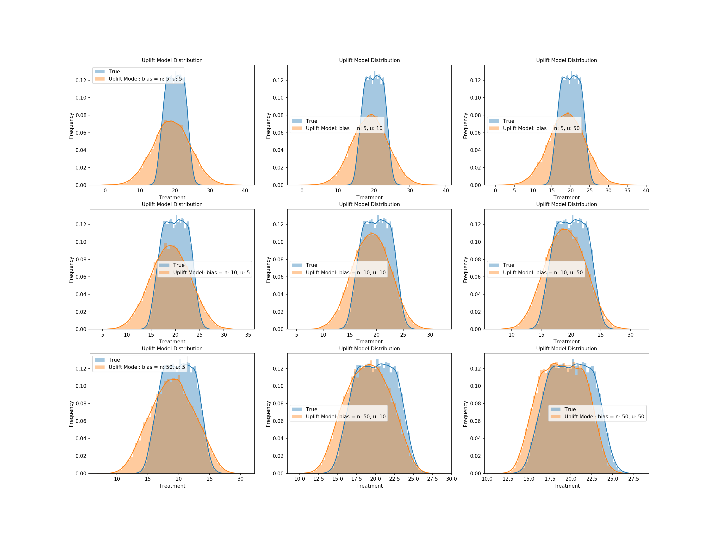
We see from above that higher scalers of the normal distribution noise contribute to an uplift that better matches the distribution of our true treatment effect - specifically the range of values - and uniform noise corrects more for the shape, but only with appropriate levels of normal noise.
The Effect of Bias and Distributional Noise vs. ATE and Profit
The steps to check the effect of the uplift model's bias as well as normal and uniform noise on our results follow. We will run trials and keep an uplift model if its mean is within 80% of the true treatment effect. Steps are as follows:
- Randomized values for bias and the scalers on the normal and uniform components are generated
- The predicted treatment effect for the corresponding uplift model is derived
- The created uplift model is categorized into bins for 10-20% less than the true treatment effect's mean, 0-10% less, 0-10% more, or 10-20% more
- 500 iterations of each range of model are generated
- These models are used to provide insights into the average ATE and profits of models given noise that produces a model in such a range
Functions used in our iterations follow.
def variable_parameter_generation():
    """
    Generates parameters for an uplift model from distributions close
    to centered around those for the iterated trials
    """
    variable_bias = random.uniform(-5, 5) # Iterated trial value = -1
    variable_normal_scale = random.uniform(1, 100) # Iterated trial value = 50
    variable_uniform_scale = random.uniform(1, 100) # Iterated trial value = 50

    return variable_bias, variable_normal_scale, variable_uniform_scale
def variable_parameter_uplift(bias, normal_scale, uniform_scale):
    """
    Generates an uplift model, and checks what the ratio
    of treatment effect for the generated uplift model
    is in comparison to the true value - for categorization
    """
    variable_pred_uplift = generate_uplift(bias, normal_scale, uniform_scale)

    variable_pred_uplift = np.where(variable_pred_uplift<0, 0, variable_pred_uplift)
    uplift_avg_treatment = variable_pred_uplift.mean()

    # Derive relation to true treatment effect
    percent_of_true_treatment = uplift_avg_treatment/true_treatment_effect.mean()

    return variable_pred_uplift, percent_of_true_treatment
def variable_parameter_profit_ate(pred_uplift):
    """
    Computes the profit and the ATE of a PST model given
    a predicted uplift

    Process follows that of a PST within the iterated trials
    """
    assigned_prop_scores = assign_prop_scores(pred_uplift)
    assigned_prop_scores = (((assigned_prop_scores)*0.90)+0.05)

    pst_ratio=0.8
    pst_indices = np.random.choice(np.arange(y_0.size),
                                   size=int(N*pst_ratio),
                                   replace=False,
                                   p=assigned_prop_scores/assigned_prop_scores.sum())

    pst_mask = np.zeros(y_0.size, dtype=bool)
    pst_mask[pst_indices] = True

    # Weights for targeted
    weights_targeted, weights_not_targeted = targeted_pst_weight(assigned_prop_scores, pst_mask)

    pst_outcome = y_0.copy()
    pst_outcome[pst_mask] = y_1[pst_mask].copy()

    variable_pst_profit = pst_outcome.sum()-(pst_mask.mean()*N*price_of_treatment)

    variable_pst_ate = pst_weighted_ate(pst_outcome,
                                        pst_mask,
                                        weights_targeted,
                                        weights_not_targeted)

    return variable_pst_profit, variable_pst_ate
def in_range_assignment(num_assigned, range_vals, percent_of_true_treatment,
                        profit_list, var_profit,
                        ATE_list, var_ATE,
                        parameters_list, var_bias, var_norm, var_uniform,
                        notify_1, notify_2):
    """
    Allows for easy assignment of values to ranges determined
    by the ratio of the uplift that generates them to the true treatment
    """
    if num_assigned < trials_per_range: # Same number of each range of model is collected
        if range_vals[0]<percent_of_true_treatment<=range_vals[1]: # Within a range of the true treatment effect
            profit_list.append(var_profit) # Assign profit
            ATE_list.append(var_ATE) # Assign ATE
            parameters_list.append([var_bias, var_norm, var_uniform]) # Save parameters
            num_assigned += 1
            if num_assigned % 100 == 0:
                print('{}% of models in {} to {}% range found.'.format(int(num_assigned/5),
                                                                         notify_1,
                                                                         notify_2))

    return num_assigned, profit_list, ATE_list, parameters_list
The following cell runs our trials, categorizes them based on the mean of their predicted uplift, and saves diagnostics such as price, ATE, and the selected parameters per trial.
At the end we will present the average bias, normal scale, and uniform scale within each range of uplift accuracy.
num_trial_20_10 = 0
num_trial_10_0 = 0
num_trial_0_10 = 0
num_trial_10_20 = 0
num_trial_out_of_range = 0

profits_20_10 = []
profits_10_0 = []
profits_0_10 = []
profits_10_20 = []

ATE_20_10 = []
ATE_10_0 = []
ATE_0_10 = []
ATE_10_20 = []

parameters_20_10 = []
parameters_10_0 = []
parameters_0_10 = []
parameters_10_20 = []

stop_binary = 0
trials_per_range = 500

while stop_binary == 0:

    # Produce variable uplift model parameters
    variable_bias, variable_normal_scale, variable_uniform_scale = variable_parameter_generation()

    # Get uplift and its relation to the true treatment effect
    variable_pred_uplift, percent_of_true_treatment = variable_parameter_uplift(variable_bias,
                                                                                variable_normal_scale,
                                                                                variable_uniform_scale)

    # Derive profit and the ATE of the trial
    variable_pst_profit, variable_pst_ate = variable_parameter_profit_ate(variable_pred_uplift)

    # Assign values to ranges of relation to the true treatment effect
    # -20 to -10%
    num_trial_20_10, profits_20_10, ATE_20_10, parameters_20_10 = in_range_assignment(num_trial_20_10, [0.8, 0.9], percent_of_true_treatment,
                                                                                      profits_20_10, variable_pst_profit,
                                                                                      ATE_20_10, variable_pst_ate,
                                                                                      parameters_20_10, variable_bias, variable_normal_scale, variable_uniform_scale,
                                                                                      '-20', '-10')
    # -10 to 0%
    num_trial_10_0, profits_10_0, ATE_10_0, parameters_10_0 = in_range_assignment(num_trial_10_0, [0.9, 1], percent_of_true_treatment,
                                                                                  profits_10_0, variable_pst_profit,
                                                                                  ATE_10_0, variable_pst_ate,
                                                                                  parameters_10_0, variable_bias, variable_normal_scale, variable_uniform_scale,
                                                                                  '-10', '0')
    # 0 to 10%
    num_trial_0_10, profits_0_10, ATE_0_10, parameters_0_10 = in_range_assignment(num_trial_0_10, [1, 1.1], percent_of_true_treatment,
                                                                                  profits_0_10, variable_pst_profit,
                                                                                  ATE_0_10, variable_pst_ate,
                                                                                  parameters_0_10, variable_bias, variable_normal_scale, variable_uniform_scale,
                                                                                  '0', '10')
    # 10 to 20%
    num_trial_10_20, profits_10_20, ATE_10_20, parameters_10_20 = in_range_assignment(num_trial_10_20, [1.1, 1.2], percent_of_true_treatment,
                                                                                      profits_10_20, variable_pst_profit,
                                                                                      ATE_10_20, variable_pst_ate,
                                                                                      parameters_10_20, variable_bias, variable_normal_scale, variable_uniform_scale,
                                                                                      '10', '20')
    # Out of 80% accuracy
    if percent_of_true_treatment<=0.8 or percent_of_true_treatment>1.2:
        num_trial_out_of_range += 1

    # Stop criteria
    if num_trial_20_10 == trials_per_range and num_trial_10_0 == trials_per_range and num_trial_0_10 == trials_per_range and num_trial_10_20 == trials_per_range:
        stop_binary = 1

print('-----')
print('Trials outside -20 to 20%: {}'.format(num_trial_out_of_range))
Let's now inspect the averages within the given ranges.
def avg_parameter_in_scale(list_of_range_parameter_lists, index, trials_per_range):
    """
    Allows us to easily seperate all iterations of bias, normal noise,
    and uniform noise from a list of lists

    Returns: the average of the parameter in the range
    """
    parameters = [l[index] for l in list_of_range_parameter_lists]
    avg = round(sum(parameters)/trials_per_range,2)

    return avg
# Calculate the average of each parameter in the given range
bias_20_10 = avg_parameter_in_scale(parameters_20_10, 0, trials_per_range)
bias_10_0 = avg_parameter_in_scale(parameters_10_0, 0, trials_per_range)
bias_0_10 = avg_parameter_in_scale(parameters_0_10, 0, trials_per_range)
bias_10_20 = avg_parameter_in_scale(parameters_10_20, 0, trials_per_range)

norm_20_10 = avg_parameter_in_scale(parameters_20_10, 1, trials_per_range)
norm_10_0 = avg_parameter_in_scale(parameters_10_0, 1, trials_per_range)
norm_0_10 = avg_parameter_in_scale(parameters_0_10, 1, trials_per_range)
norm_10_20 = avg_parameter_in_scale(parameters_10_20, 1, trials_per_range)

uniform_20_10 = avg_parameter_in_scale(parameters_20_10, 2, trials_per_range)
uniform_10_0 = avg_parameter_in_scale(parameters_10_0, 2, trials_per_range)
uniform_0_10 = avg_parameter_in_scale(parameters_0_10, 2, trials_per_range)
uniform_10_20 = avg_parameter_in_scale(parameters_10_20, 2, trials_per_range)
# Make a df with the base results
df_base_trial_results = pd.DataFrame(columns = ['Range', 'Iterations', 'Avg Bias', 'Avg Norm Scale', 'Avg Uniform Scale'])

df_base_trial_results['Range'] = ['-20 to -10%', '-10 to 0%', '0 to 10%', '10 to 20%']
df_base_trial_results['Iterations'] = [num_trial_20_10, num_trial_10_0, num_trial_0_10, num_trial_10_20]
df_base_trial_results['Avg Bias'] = [bias_20_10, bias_10_0, bias_0_10, bias_10_20]
df_base_trial_results['Avg Norm Scale'] = [norm_20_10, norm_10_0, norm_0_10, norm_10_20]
df_base_trial_results['Avg Uniform Scale'] = [uniform_20_10, uniform_10_0, uniform_0_10, uniform_10_20]

display(df_base_trial_results)
From the above we can see that bias has the most dramatic effect on the accuracy of the uplift model, so much so that the effects of the distributional scalers are mitigated. We'll save the average profits and average treatment effects till the end where we will compare them to the prior results to see if they fall close to the results we got before the the normal PST trial.
As a final graphical check, we look into the following:
- The profits (and ATEs) of trials across our accuracy ranges
- The relation between bias and profit (or ATE) across trials
- The relation between normal noise and profit (or ATE) across trials
- The relation between uniform noise and profit (or ATE) across trials
We'll first bin results so it's easier to view them graphically.
def bin_list_and_average_bins(list_of_vals, total, bin_len):
    """
    Bins values within a large list into a list of lists, then finds the
    averages of the bins for graphing
    """
    list_binned = [list_of_vals[i:i+bin_len] for i in range(0, total, bin_len)]
    list_of_bin_avgs = [sum(i)/bin_len for i in list_binned]

    print('Length of new list:', len(list_of_bin_avgs))

    return list_of_bin_avgs
bin_len = 10

# Bin and average bins of profit lists
profits_20_10_binned_avgs = bin_list_and_average_bins(profits_20_10, len(profits_20_10), bin_len)
profits_10_0_binned_avgs = bin_list_and_average_bins(profits_10_0, len(profits_10_0), bin_len)
profits_0_10_binned_avgs = bin_list_and_average_bins(profits_0_10, len(profits_0_10), bin_len)
profits_10_20_binned_avgs = bin_list_and_average_bins(profits_10_20, len(profits_10_20), bin_len)

# Bin and average bins of ATE lists
ATE_20_10_binned_avgs = bin_list_and_average_bins(ATE_20_10, len(ATE_20_10), bin_len)
ATE_10_0_binned_avgs = bin_list_and_average_bins(ATE_10_0, len(ATE_10_0), bin_len)
ATE_0_10_binned_avgs = bin_list_and_average_bins(ATE_0_10, len(ATE_0_10), bin_len)
ATE_10_20_binned_avgs = bin_list_and_average_bins(ATE_10_20, len(ATE_10_20), bin_len)
In order to derive the effect of individual parameters on profit (or ATE), we'll combine results from across the ranges and order both them and their resulting result metrics.
def list_of_parameter_profit_or_ate(list_of_parameter_lists_1, ate_or_profit_1,
                                    list_of_parameter_lists_2, ate_or_profit_2,
                                    list_of_parameter_lists_3, ate_or_profit_3,
                                    list_of_parameter_lists_4, ate_or_profit_4,
                                    index):
    """
    Creates lists of paramter values and profits (or ATEs) sorted by the parameters for graphing

    - Bias: 0
    - Normal scale: 1
    - Uniform scale: 2
    """
    # The parameter in question is first selected using its list of lists index, and then matched with its profit (or ATE)
    ate_or_profit_20_10 = [([l[index] for l in list_of_parameter_lists_1][i], ate_or_profit_1[i]) for i in list(range(trials_per_range))]
    ate_or_profit_10_0 = [([l[index] for l in list_of_parameter_lists_2][i], ate_or_profit_2[i]) for i in list(range(trials_per_range))]
    ate_or_profit_0_10 = [([l[index] for l in list_of_parameter_lists_3][i], ate_or_profit_3[i]) for i in list(range(trials_per_range))]
    ate_or_profit_10_20 = [([l[index] for l in list_of_parameter_lists_4][i], ate_or_profit_4[i]) for i in list(range(trials_per_range))]

    # Full list of all parameter and profit (or ATE) pairs
    parameter_with_ate_or_profit_list = ate_or_profit_20_10 + ate_or_profit_10_0 + ate_or_profit_0_10 + ate_or_profit_10_20
    print('Number of elements in list:', len(parameter_with_ate_or_profit_list))

    # Order by the parameter values
    parameter_with_ate_or_profit_sorted = sorted(parameter_with_ate_or_profit_list, key=lambda tup: tup[0])

    # Seperate them and return for binning and graphing
    parameter_list, ate_or_profit_list = zip(*parameter_with_ate_or_profit_sorted)

    return parameter_list, ate_or_profit_list
The values found above are then sorted so that their effect on the ATE and profit can be derived.
# Bin each of the parameters and the corresponding profit (or ATE), then average the bins
parameter_bins = 5

bias_sort_binned = bin_list_and_average_bins(bias_sort, len(bias_sort), parameter_bins)
norm_sort_binned = bin_list_and_average_bins(norm_sort, len(bias_sort), parameter_bins)
uniform_sort_binned = bin_list_and_average_bins(uniform_sort, len(bias_sort), parameter_bins)

bias_profit_sort_binned = bin_list_and_average_bins(bias_profit_sort, len(bias_sort), parameter_bins)
norm_profit_sort_binned = bin_list_and_average_bins(norm_profit_sort, len(bias_sort), parameter_bins)
uniform_profit_sort_binned = bin_list_and_average_bins(uniform_profit_sort, len(bias_sort), parameter_bins)

bias_ATE_sort_binned = bin_list_and_average_bins(bias_ATE_sort, len(bias_sort), parameter_bins)
norm_ATE_sort_binned = bin_list_and_average_bins(norm_ATE_sort, len(bias_sort), parameter_bins)
uniform_ATE_sort_binned = bin_list_and_average_bins(uniform_ATE_sort, len(bias_sort), parameter_bins)
We now plot the following:
- Profit across trials within uplift accuracy ranges
- The relation of bias normal noise and uniform noise to profit, including a line of best fit and its equation for each
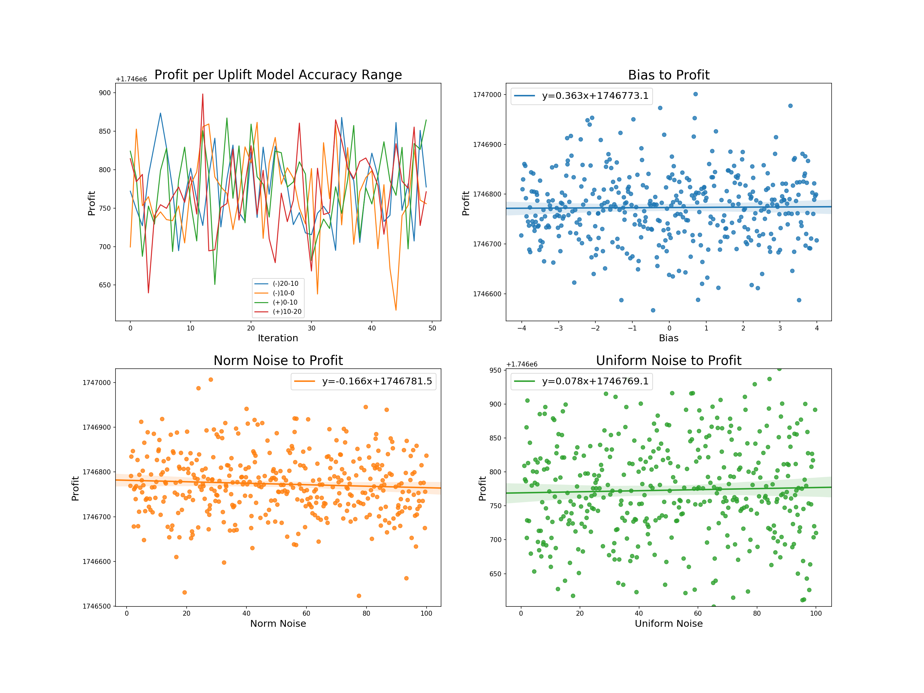
We can derive the following from the graphs:
- Profit per uplift range: there appears to be no direct relation between the degree of accuracy of the uplift model to its resulting profit.
- Bias to profit: a slight positive relationship with the highest of the intercepts. Allowing for larger biases would likely increase the slope, but such models would be more likely to fall outside of our accepted uplift range.
- Norm and uniform noise to profit: almost the exact same relation - each with a slightly higher slope than bias.
The same is displayed for ATEs:
- ATE across trials within uplift accuracy ranges
- The relation of bias normal noise and uniform noise to ATE, including a line of best fit and its equation for each
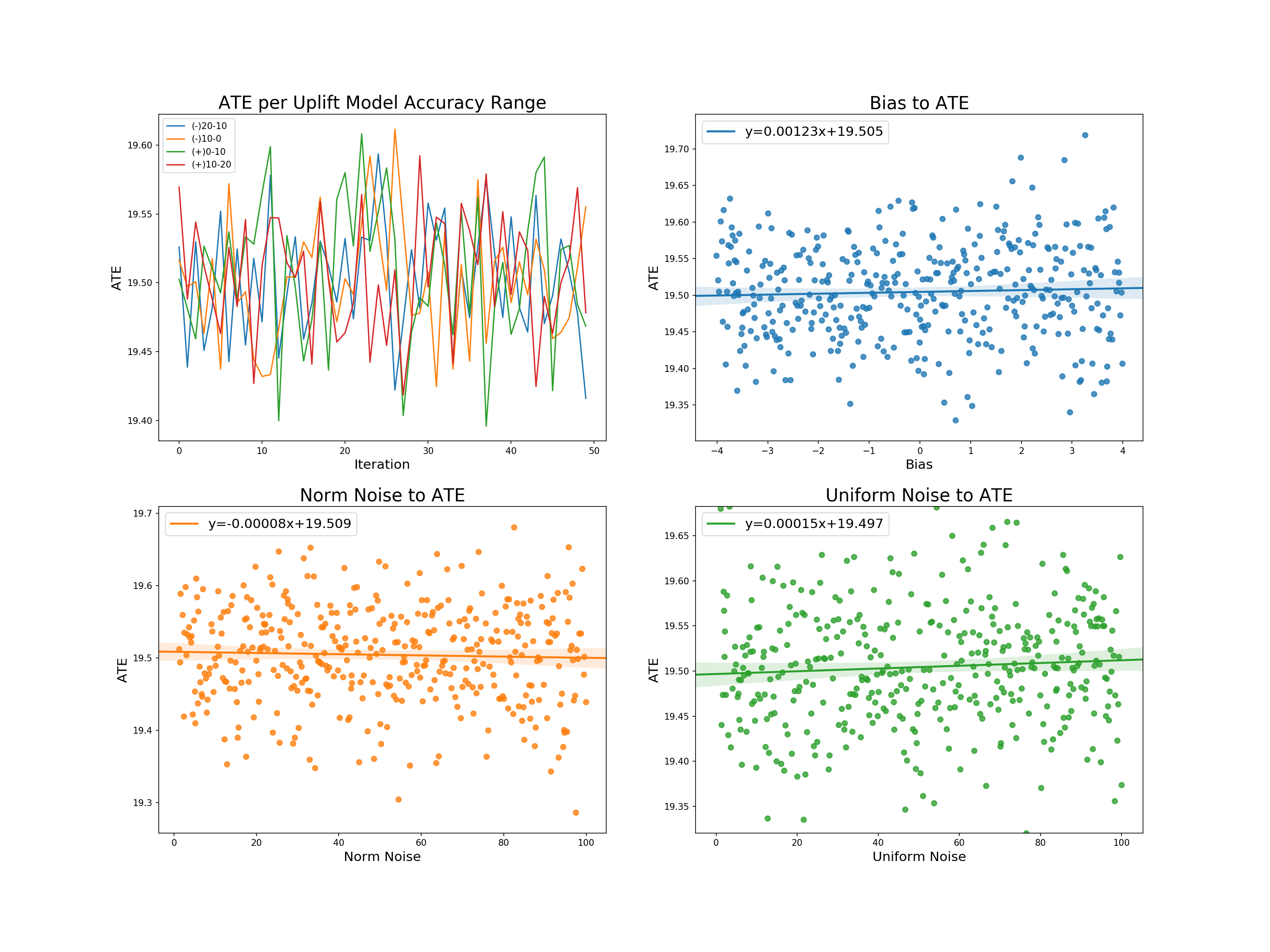
From these graphs we can further derive:
- Profit per uplift range: as with price, no degree of uplift inaccuracy can seems to have a particular effect on the average treatment effect.
- Bias, normal noise, and uniform noise to profit: each has almost the exact same linear relation to the ATE - that being no relation with an intercept reflecting the true treatment effect.
We now add the rows created on PSTs within certain model accuracy ranges to those of the original results for a final check.
# Make a results df so the previous can be appended
results_df_effects = pd.DataFrame(columns=['PST_20_10_ATE', 'PST_20_10_PI',
                                           'PST_10_0_ATE', 'PST_10_0_PI',
                                           'PST_0_10_ATE', 'PST_0_10_PI',
                                           'PST_10_20_ATE', 'PST_10_20_PI'], dtype = 'float')
# Add rows to results df
results_df_effects['PST_20_10_PI'] = profits_20_10
results_df_effects['PST_20_10_ATE'] = ATE_20_10
results_df_effects['PST_10_0_PI'] = profits_10_0
results_df_effects['PST_10_0_ATE'] = ATE_10_0
results_df_effects['PST_0_10_PI'] = profits_0_10
results_df_effects['PST_0_10_ATE'] = ATE_0_10
results_df_effects['PST_10_20_PI'] = profits_10_20
results_df_effects['PST_10_20_ATE'] = ATE_10_20
# Get columns
ATE_columns = [e for e in results_df_effects.columns if 'ATE' in e]
PI_columns = [e for e in results_df_effects.columns if 'PI' in e]
# Take absolute value of deviation of estimated ATE from true ATE
results_df_effects[ATE_columns] -= true_treatment_effect.mean()
results_df_effects[ATE_columns] = results_df_effects[ATE_columns].abs()

results_df_ate_effects = results_df_effects[ATE_columns].copy()
results_df_pi_effects = results_df_effects[PI_columns].copy()/1000 #In thousands of dollars for better readability
# Make ATE table
results_df_ate_effects_summary = results_df_ate_effects.agg(['mean','std' , 'min', 'max']).T.sort_values(by='mean')
results_df_ate_effects_summary.index = [e[:-4] for e in results_df_ate_effects_summary.index]
# Make PI table
results_df_pi_effects_summary = results_df_pi_effects.agg(['mean','std', 'min', 'max']).T.sort_values(by='mean', ascending=False)
results_df_pi_effects_summary.index = [e[:-3] for e in results_df_pi_effects_summary.index]
results_df_ate_compare = pd.concat([results_df_ate_summary, results_df_ate_effects_summary])
results_df_pi_compare = pd.concat([results_df_pi_summary, results_df_pi_effects_summary])

results_df_ate_compare = results_df_ate_compare.sort_values(by='mean')
results_df_pi_compare = results_df_pi_compare.sort_values(by='mean', ascending=False)
A base result looking at the average treatment effect diagnostics shows us that PST trials have a similar average treatment effect to one another, with those trials that have models constricted to one range having slightly lower effects than a group that draws multiple times using bias = -1, and the scalers on norm and uniform noise being 50. Significantly, none of the range based PST trial groups have averages that would give them more or less of an effect to any other style of trial.
The profits above are scaled to 1000s of dollars for readability. We see propensity score targeting with controlled ratio targeting provides the highest average return, more so than the imbalanced tests, as we have selected individuals at the higher end of propensity weighting more, and thus realized their higher returns while maintaining balance across the propensity distribution. The standard deviation is of course higher based on propensity derivation, but overall the model performs well in maximizing profits.
The alternative and rescaled propensity targeting tests both return less average profit than the 80% imbalanced trials, but more than the conventional RCT. This implies that in these cases the uplift generated propensity wasn't accounted for enough in selection, which makes sense given PST_ALT being randomized, and the scaled model losing its distributional tails.
With further regard to the rescaled propensity targeting, it should be noted that the chosen scaling distribution will have effects on its average profits, as previous model runs with ranges scaled to [0.25, 0.75] provided less average profit than IMB_06. The very low standard deviation of PST_RESC could be a general positive for a practitioner if it weren't for its under-performance to even IMB_08 in terms of profit. A balance between the profit maximization of a normal PST model and which degree of scaling would allow for more assured results could be further found.
Results and Outlook
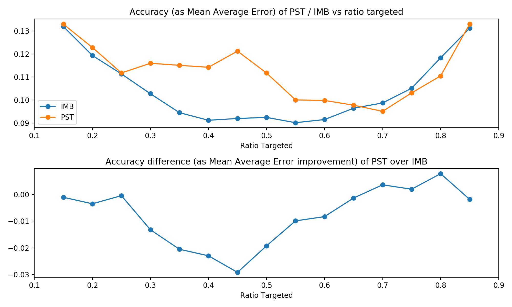
We simulated both approachs for different target ratios. Since we do not allow propensity scores outside of [0.1, 0.9] to avoid having extreme scores giving individual samples enormous weights, we limited our target ratios to [0.15, 0.85]. This ensures that the variation in our propensity scores is always at least 10%. For each ratio, we simulated both approaches 500 times to ensure that we get robust representative results.
Both traditional imblanced targeting and our propensity score targeting are first and foremost techniques for estimating the average treatment effect. The table below shows that the accuracy of proper randomised trials is consistently better than our PST technique. This is not completely unexpected. However, those differences are pretty negligible: Our true population ATE is 20, while the worst difference in MAE between the two techniques was about 0.03, or about 0.15% of the treatment effect. So both techniques performed very similar.
One noticable trend is that the two approaches performed most similar at the extreme ends of the proportion targeted. This is caused by our propensity score algorithm. Recall that it always chooses the maximum variation in scores possible, and that this is larger the closer the target ratio is to 0.5. Thus, at the extreme ends of the target proportions, there isn't too much variation in propensity scores and thus PST acts most similar to a normal RCT with imbalanced targeting.
When it comes to profit increases, a similar trend emerges. Recall that treatment is strictly profitable in our case, so a higher proportion target implies higher profits. Thus, both curves are strictly increasing. And similarly to the accuracy of the estimates, the two techniques performed more similar the closer they are to the extreme of percentage targeted. At 0.5, where PST is allowed the greatest variation, it outperforms a classical RCT the most.
Overall, these results are quite promising: They show that both techniques lead to a similar accuracy in their estimates of the ATE, while also showing that PST is more profit-efficient. However, those differences are pretty small and while our many iterations ensure that those are true trends, it seems that PST does not add too much at present.
One avenue for improvement seems promising: Adding more variation to the propensity scores of PST even at more extreme targeting ratios might drastically improve the profit-performance. Currently, we force the propensity scores into a uniform distribution. The advantage of that is that it should be relatively easy to force this uniform distribution into another, more extreme distribution in the same interval. We could for instance map it to a bimodal distribution with the same mean, and thus might improve our results.
Appendix: More extreme propsensity scores
Let's briefly test two spinds of our propensity score assignment procedure that lead to less extreme scores: first, setting all scores higher than the mean to the maximum score and all scores lower than the mean to the minimum scores; second, same as above, but instead we set scores to the 25th and 7th quantile instead. See the code and plots below for how they work.
Note that our predicted uplift is a nice, symmetric normal distribution. However, since we map predicted uplift to a uniform distribution first, we are always guaranteed to end up with a symmetric distribution, too. Thus, these new scaling procecures are certain to be mean-preserving.
ratio = 0.8
ordered =  sp.stats.rankdata(pred_uplift)-1
ordered = ordered / ordered.size
max_len = min( (ratio - 0.1) * 2 , (0.9 - ratio) * 2 )
ordered = ordered * max_len
assigned_prop_scores = ordered + (ratio - ordered.mean())

# for min max scaling
minscore = assigned_prop_scores.min()
maxscore = assigned_prop_scores.max()
assigned_prop_scores = np.where(assigned_prop_scores > ratio,maxscore, minscore)

# for quantile scaling
minscore = np.quantile(assigned_prop_scores, 0.25)
maxscore = np.quantile(assigned_prop_scores, 0.75)
assigned_prop_scores = np.where(assigned_prop_scores > ratio,maxscore, minscore)

We can see that the most extreme min-max scaling performs best in terms of profit and slightly worse in terms of accuracy, while quantile scaling is the most consistent but gains less profit over normal imbalanced targeting. So as we might have expected, there is a trade-off between accuracy and profit-increase.
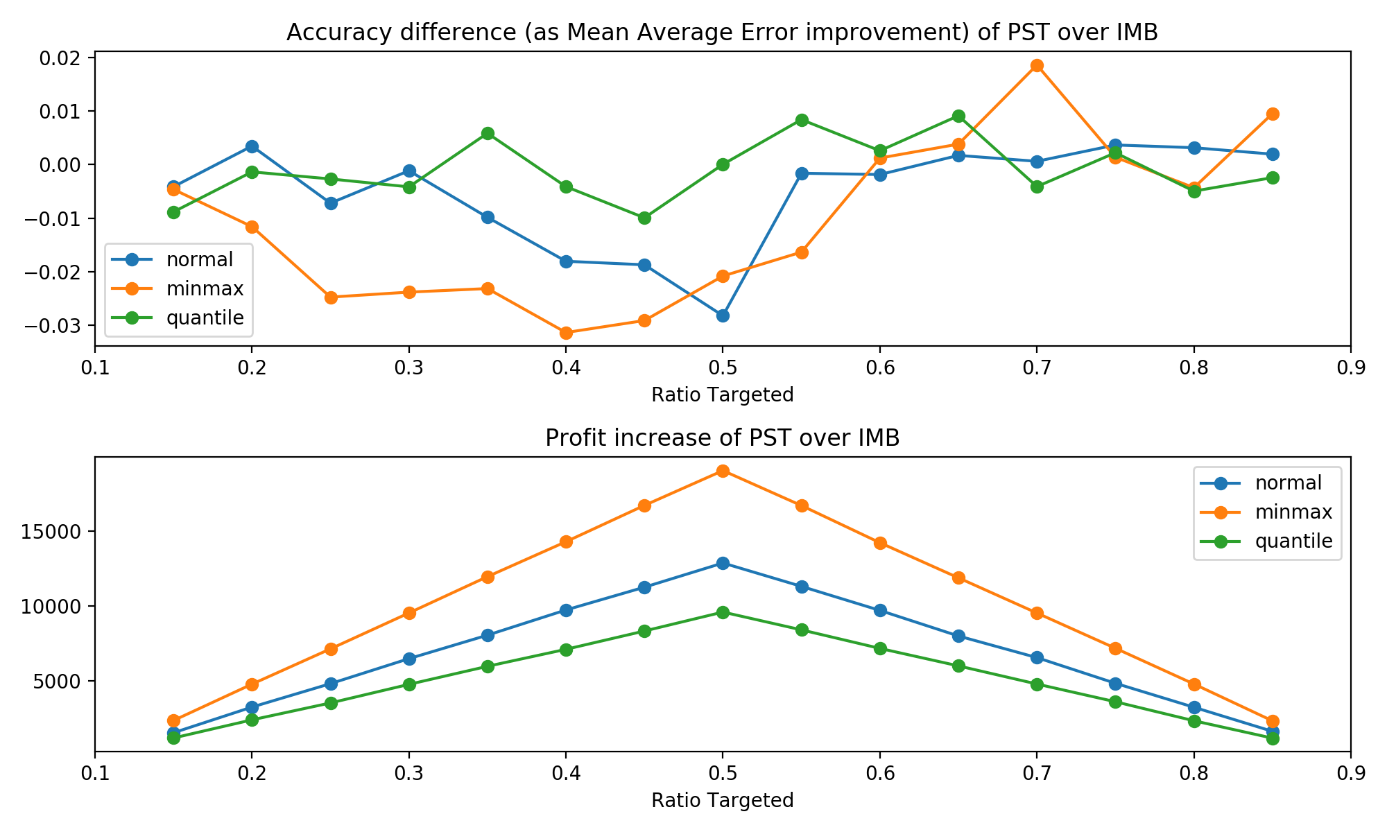
Now, our procedure is only preserving the ordering of predicted uplift scores, but information about the original distribution is lost. Maybe mapping the predicted uplift scores to propensity scores in a way that preserves this information can offer some improvement. However, this would add further complexity in case the distribution of predicted uplift is not symmetric.
As a side note: All approaches perform quite similar at the higher end of targeting ratios in terms of accuracy. We conjecture that this is caused by our uplift model being simulated as biased. (See plots below.)
sns.distplot(pred_uplift, label = 'Uplift Model')
sns.distplot(true_treatment_effect, label = 'True Teatment Effect')
plt.legend()
plt.show()

Sources
- Angrist, J. D., & Pischke, J.-S. (2009). Mostly harmless econometrics: An empiricist's companion. Princeton: Princeton University Press.
- Auer, P., Cesa-Bianchi, N. & Fischer, P. Machine Learning (2002) 47: 235. https://doi.org/10.1023/A:1013689704352
- Bouneffouf D., Bouzeghoub A., Gançarski A.L. (2012) A Contextual-Bandit Algorithm for Mobile Context-Aware Recommender System. In: Huang T., Zeng Z., Li C., Leung C.S. (eds) Neural Information Processing. ICONIP 2012. Lecture Notes in Computer Science, vol 7665. Springer, Berlin, Heidelberg.
- Farrell, M., Liang, T., & Misra S. (2018). Deep Neural Networks for Estimation and Inference: Application to Causal Effects and Other Semiparametric Estimands. Draft version December 2018, arXiv:1809.09953, 1-54.
- Hitsch, G J. & Misra, S. (2018). Heterogeneous Treatment Effects and Optimal Targeting Policy Evaluation. January 28, 2018, Available at SSRN: https://ssrn.com/abstract=3111957 or http://dx.doi.org/10.2139/ssrn.3111957
- Imbens, G. W., & Wooldridge, J. M.(2009). Recent Developments in the Econometrics of Program Evaluation. Journal of Economic Literature, 47 (1): 5-86.
- King, G., & Nielsen, R. (2019). Why Propensity Scores Should Not Be Used for Matching. Political Analysis. Draft version November 2018, 1-33. Copy at http://j.mp/2ovYGsW
- Lachin, J. M. (1988). Statistical properties of randomization in clinical trials. Controlled Clinical Trials. Volume 9, Issue 4, December 2988, 289-311.
- Lachin, J. M., Matts, J. P., Wei, L. J. (1988). Randomization in clinical trials: Conclusions and recommendations. Controlled Clinical Trials. Volume 9, Issue 4, December 1988, 365-374.
- Lambert, B. (2014, Feb 7). Propensity score - introduction and theorem. Retrieved from https://www.youtube.com/watch?v=s1YpulokvEQ
- Lambert, B. (2014, Feb 7). Propensity score matching: an introduction. Retrieved from https://www.youtube.com/watch?v=h0UU6trKR0E
- Lambert, B. (2014, Feb 7). Propensity score matching - mathematics behind estimation. Retrieved from https://www.youtube.com/watch?v=S_2Al_v3oK4
- Langford, J., Zhang, T. (2008), "The Epoch-Greedy Algorithm for Contextual Multi-armed Bandits", Advances in Neural Information Processing Systems 20, Curran Associates, Inc., pp. 817–824.
- Li F., Morgan, K L & Zaslavsky, A M. (2018). Balancing Covariates via Propensity Score Weighting. Journal of the American Statistical Association, 113:521, 390-400, DOI: 10.1080/01621459.2016.1260466
- McCaffrey, D. F., Ridgeway, G., & Morral, A. R. (2004). Propensity Score Estimation With Boosted Regression for Evaluating Causal Effects in Observational Studies. Psychological Methods, 9(4), 403-425. http://dx.doi.org/10.1037/1082-989X.9.4.403
- Meldrum, M. L. (2000). A Brief History of the Randomized Controlled Trial: From Oranges and Lemons to the Gold Standard. Hematology/Oncology Clinics of North America, August 2000, 745-760.
- Rosenbaum, P. & Rubin, D. (1983). The central role of the propensity score in observational studies for causal effects. Biometrika, 70, 41-55.
- Rosenbaum P.R. (2002). Overt Bias in Observational Studies. In: Observational Studies. Springer Series in Statistics. Springer, New York, NY
- Rosenberger, W. F., Lachin, J. M. (1993). The use of response-adaptive designs in clinical trials. Controlled Clinical Trials. Volume 14, Issue 6, December 1993, 471-484.
- Rubin, D. B. (1990). Formal Modes of Statistical Inference for Causal Effects, Journal of Statistical Planning and Inference.
- Rubin, D. B. (1980). Randomization Analysis of Experimental Data: The Fisher Randomization Test Comment, Journal of the American Statistical Association, 75, 591–593.
- Schnabel, T. et al. (2016). Recommendations as Treatments: Debiasing Learning and Evaluation. Draft version May 2016, arXiv:1602.05352, 1-10.
- Schulz, K. F., Grimes, D. A. (2002). Generation of allocation sequences in randomised trials: chance, not choice. The Lancet, Volume 359, Issue 9305, February 2002, 515-519.
- Tokic M. (2010) Adaptive ε-Greedy Exploration in Reinforcement Learning Based on Value Differences. In: Dillmann R., Beyerer J., Hanebeck U.D., Schultz T. (eds) KI 2010: Advances in Artificial Intelligence. KI 2010. Lecture Notes in Computer Science, vol 6359. Springer, Berlin, Heidelberg.
- Vermorel J., Mohri M. (2005) Multi-armed Bandit Algorithms and Empirical Evaluation. In: Gama J., Camacho R., Brazdil P.B., Jorge A.M., Torgo L. (eds) Machine Learning: ECML 2005. ECML 2005. Lecture Notes in Computer Science, vol 3720. Springer, Berlin, Heidelberg.
- Weber, R. (1992) On the Gittins Index for Multiarmed Bandits. Ann. Appl. Probab. 2, no. 4, 1024--1033. doi:10.1214/aoap/1177005588.
- Zwarentein, M., Treweek, S., Gagnier, J. J., Altman, D. G., Tunis, S., Haynes, B., ... Moher, D. (2009). Improving the reporting of pragmatic trials: An extension of the CONSORT statement. Journal of Chinese Integrative Medicine, 7(4), 392-397.