By Julian Winkel, Tobias Krebs | August 18, 2019
Data Generating Process Simulation
Introduction
Topic
As modern science becomes increasingly data-driven among virtually all fields, it is obligatory to inspect not only how scientists analyze data but also what kind of data is used. Naturally, the performance of a model is bound by the quality of underlying data. This blog post explores the properties and constituents of realistic data sets and proposes flexible and user-friendly software to support research by means of 'Simulated Data Generating Processes' (SDGP).
Motivation
With increasing dimension, standard Machine Learning Techniques tend to suffer from the 'Curse of Dimensionality', referring to the phenomenon of data points becoming sparse for constant sample sizes, whilst large parameter spaces render consistent estimation difficult (Chernozhukov, 2017). However, having more and more data available, these problems need to be addressed in a specialized framework. Facing ever growing amounts of data in different fields of interests in statistics and econometrics, e.g. inference, time series analysis, causality or prediction, the necessity of generating flexible data sets becomes obvious. Especially when dealing with methods such as Neural Networks, which are often labelled as 'Black Boxes', model reactions to data changes are particularly insightful.
Properties
The researcher's setting is located in a high-dimensional, partial-linear model. The covariates are pseudo-randomly generated in such a manner that they are (partially) correlated with the output variable, which itself can take binary or continuous values. The relation between the covariates and the output variable can be specified as linear or non-linear. Individual treatment assignment, propensity, being the probability of treatment assignment, can be random or non-random. One of the fundamental problems researchers face is the non-observability of counterfactuals and treatment effects, firstly addressed in the 'Potential Outcomes Framework' (Rubin, 2011). In the proposed setting, treatment effects are known and can be customized in their effect. By proposing a model in which all components are expounded, researchers receive support to evaluate and compare various models that are applied to a realistic data set.
Review
Literature
Chernozhukov et al. address some problems in the area of modern, prediction focussed machine learning. Using Robinson's framework, they argue, standard techniques to estimate statistics as 'regression coefficients, average treatment effects, average lifts, and demand or supply elasticities' can easily fail due to regularization bias. They suggest to estimate and compensate the introduced bias in a double machine learning setting in order to restrict estimated parameters to a reasonably small space. The resulting estimators are proven to have desirable statistical properties; hence presenting a method to apply common machine learning methods as 'random forest, lasso, ridge, deep neural nets, boosted trees' in a highdimensional and nonlinear model.
Powers et al. are handling high dimensional, observational data and try to estimate treatment effects. They target regions of especially high or low treatment effects in the parameter space, for their average might be close to zero. Having proposed various models to estimate heterogeneous treatment effects, they simulate a data set that mimics their original data in order to compare model performance.
Dorie et al. compare inferential strategies from a data analysis competition. The authors criticize a general lack of guidance on optimal applications of statistical models. They discuss the problem of adequately assigning participants to test and control groups where unobserved characteristics require a tradeoff between a demanding parametric structure or flexibility. Results from a competition for various models and strategies are reported and compared, yielding in an overall surplus for flexibility. Moreover, they provide a list of un-addressed issues to be considered for application, including (but not limited to) non-binary treatment, non-continuous response, non-iid data, varying data / covariate size. Our proposed model accounts for the mentioned issues.
Jacob et al. provide an analysis on the application of modern machine learning techniques on simulated data; relying on a setting as in Robinson's framework. They compare different methods to estimate causal effects where the true treatment effects are known. This is the foundation of our blog post.
Software
Naturally, software packages that generate synthetic data sets already exist. Given that the most popular languages for data analysis are R and Python, it is desirable to provide the according software in the respective environment. One existing R package to deal with data generating processes is simstudy (Goldfeld, 2019).
While simstudy provides great flexibility, using low-level functions to generate desirable relationships, it comes at the cost of properly understanding their backend and the ability to create a sound statistical model with regard to the probability theoretic background. Furthermore, it is costly to create high dimensional data sets.
To enrich and broaden the state of the art, our proposed model aims to strip the user of this burden by offering a backend which can be easily accessed, but by no means has to be regarded at all by the user. Hence the informed user can decide how deeply he wants to explore the underlying mathematics. On top of the backend, we offer an easily-adjustable user interface for common scientific approaches.
Theory behind the package
In the following sections you will find a step by step explanation of how our data simulation package works internally, accompanied by the corresponding formulas, code snippets and explanatory graphs.
General Model: Partial Linear Regression
The model that our package is based on is a partial linear regression model as it is described in Chernozhukov (2017). It consists of the covariates X that are possibly non-linear in relation to y, the treatment term consisting of the treatment effect and the treatment assignment vector, and a normally distributed error term.
$Y$ - Outcome Variable $\quad \theta_0$ - True treatment effect $\quad D$ - Treatment Dummy $ \quad X_{n*k}$ - Covariates
$U$, $V$ & $W$ - normally distributed error terms with expected value 0
Generating Covariates
Continuous Covariates
The covariate matrix $X$ in our simulation is drawn from a multivariate normal distribution with an expected value of 0 and a specified covariance matrix $\Sigma$. $\Sigma$ is constructed the following way. First, values for Matrix $A$ are drawn from a uniform distribution. In a second step, to make sure that there exist negative correlations and that not all variables are highly correlated with each other, we create an overlay matrix $B$. This overlay matrix $B$ consists of values 1 and -1. Third, we multiply the two matrices element-wise and adjust the result with a correction term to assure that values in $\Sigma$ are not increasing in $k$. This result is represented by the matrix $\Lambda$. In a final step, we calculate $\Sigma$ by multiplying $\Lambda$ with its transposed to assure that it is positive definite.
With the following variables:,
$n = Number \; of \; Observations, \quad k = Number \; of \; Covariates$
$\Sigma = \Lambda*\Lambda^T, \quad \Lambda = \frac{10}{k} (A \circ B), \quad A \sim U(0,1), \quad B \sim Bernoulli(0.5)\;,B \in \{-1,1\}$
$Matrices \; A, \; B, \; and \; \Lambda \; are \; all \; of \; dimension \; k*k$
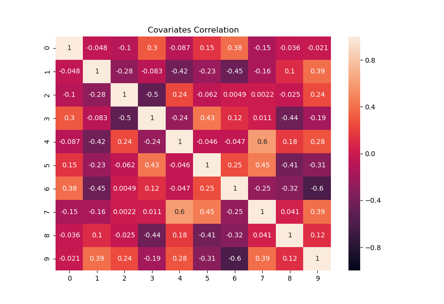
The following heat-map shows an example of Sigma with k=10 covariates. Depending on the chosen random seed, typically correlations range between -0.7 and 0.7 with slightly varying minimum and maximum values.
Binary and categorical covariates
Binary and categorical covariates are created by transforming the continuous covariates $X$. Depending on what option is chosen, the package simulates all covariates or a subset of $X$ as binary and/or categorical. The covariates are transformed by min-max-standardization to obtain prediction values. These values are then used to either obtain binary realizations from a Bernoulli distribution or categorical covariates by summing up the realizations of several Bernoulli draws.
$$ p_{j} = \frac{x(j) - min(x(j))}{max(x(j)) - min(x(j))} $$$$ x_{binary}(j) = Bernoulli\left( p_{j} \right) $$$$ x_{categorical}(j) = \sum_{c=1}^{C-1} Bernoulli_c \left( p_{j} \right) $$Where,
$x(j) \in X = covariate\; vector, \quad j \in \{1,...,k\}, \quad C = number\; of\; categories $
The following code serves as an example of how binary and categorical covariates are implemented. In this example, the user chooses how many covariates are transformed and gives a list of categories that should be included, e.g. [2,5] for binary and categorical variables with 5 categories.
Treatment assignment
There are two ways treatment can be assigned. The first one is to simulate a random control trial where all observations are assigned treatment with the same probability $m_0$. This is a rather rare case in reality since most datasets are not constructed from experiments but there still exist cases where it is a realistic assumption, e.g. medical or psychological studies. The second one is assigning treatment in the fashion of an observational study where assignment of treatment depends on covariates $X$ and probability $m_0$ differs between observations. This is the far more common case in all kinds of fields, especially in more business related cases, e.g. customers that sign up for newsletters but also people starting in job programs are not randomly selected into taking part in those programs. The assignment vector $D$ is drawn from a Bernoulli distribution with probability $m_0$ in both cases.
$$ D_{n*1} \sim Bernoulli(m_0) $$Random
In the random assignment case, only an assignment probability $m_0$ has to be chosen which is then used to draw realizations from a Bernoulli distribution to create the assignment vector $D$.
$$ m_0 \in [0,1] $$Dependent on covariates
To obtain the individual probabilities, as a first step, a subset $Z \subseteq X$ with dimensions $n$ times $l$ is chosen. Then, $Z$ is multiplied with a weight vector $b$, which is made up of values drawn from a uniform distribution, resulting in vector $a$. The standardized version of vector $a$ is then used to draw values from a Normal CDF which eventually serve as assignment probabilities in vector $m_0$. To include some randomness, random noise, drawn from a uniform distribution and labeled as $\eta$, is added to $a$ before the standardization.
Where,
$ a_{n*1} = Z * b + \eta, \quad Z_{n*l} \subseteq X_{n*k}, \quad b_{l*1} \sim U(0,1), \quad \eta_{n*1} \sim U(0,0.25)$
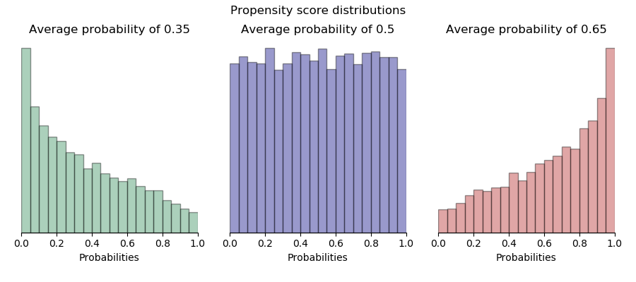
The following histograms show the distributions of propensity scores ($m_0$) in the case of non-random assignment with low, medium, and high average assignment probability. In the trivial case of random assignment, propensity scores are all the same for each observation.
Treatment effects
The package offers 6 different options for the treatment effect $\theta_0 $. These effects are: Positive constant, negative constant , positive heterogeneous, negative heterogeneous, no effect, and discrete heterogeneous. When applying these treatment effects, one can choose a single option or pick preferred options and apply a mix of them.
Positive & negative constant effect
In the case of a constant effect, treatment is the same for each individual and, thus, is just a constant $c$. Depending on the chosen sign either positive or negative. This is a popular assumption in research which can serve as a benchmark.
Option 1 positive constant: $$ \theta_0 = c $$
Option 2 negative constant: $$\theta_0 = - \; c$$
Positive & negative continuous heterogeneous effect
In contrast to the constant effect, for which each observation has the same treatment effect, the continuous heterogeneous effect differs between individuals within a specified interval. Moreover, depends the size of the individual treatment effect on a subset Z of the covariates X. That the treatment effect is different among individuals is quite common, e.g. coupons lead to different amounts of purchases or the same kind of medicine has a different effect on different patients which is due to their differing characteristics.
The creation of this treatment effect begins similar to the treatment assignment with taking the dot product of the subset $Z$ and the same weight vector used in the treatment assignment $b$. The result is forwarded into a sine function and a normally distributed error term $W$ is added. The result $\gamma$ is then min-max-standardized and adjusted in size with a constant $c$. Note that eventually the size of treatment depends on the intensity chosen which will be explained later on in the Package application part. In case that the heterogeneous effect is supposed to be partly or entirely negative, the resulting distribution is shifted by the respective quantile value $q_{neg}$ that corresponds to the wanted negative percentage share.
Where,
$Z \subseteq X,\quad b_{k*1} \stackrel{ind.}{\sim} U(0,1), \quad W \stackrel{ind.}{\sim} N(0,1), \quad q_{neg} \in [0,c], \quad c = size \; adjustment \; parameter$
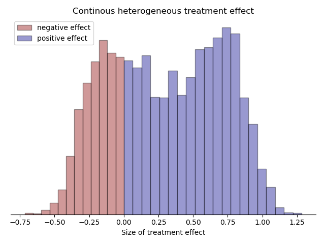
The following histogram shows an example where 30% of the continuous heterogeneous treatment effect is negative and 70% is positive.
No effect
This option allows that there are cases of treatment assignment that show no effect, i.e. $\theta_0$ is simply 0.
This could be the case e.g. when customers are target with some kind of commercial that does not reach them due to logistic reasons.
Discrete heterogeneous treatment effect
The discrete heterogeneous treatment effect is created in a similar manner as the continuous version. The scalar product of a subset of the covariates is put into a sinus function and the result is standardized to be interpretable as a probability. In another step, those probabilities are used to draw values from a Bernoulli distribution, where 0's are exchanged with the lower value and 1's with the higher value of the new treatment effect. The resulting treatment effect depends then on a subset of covariates.
$$\gamma = sin(Z * b)$$$$ p_{dh} = \frac{\gamma - min(\gamma)}{max(\gamma) - min(\gamma)}$$$$ \theta_0 \sim Bernoulli(p_{dh}), \; \theta_0 \in \{0.1*c , 0.2*c\}$$Output variable
Continuous
The continuous output variable $Y$ comprises of three main parts. The treatment part $\theta_0 D $ as explained above, the possibly non-linearly transformed covariates $X$, and the error term $U$. The transformation $g_0()$ consists of two parts. First, the dot product of $X$ and the weighting vector $b$ is taken. The values of $b$ are drawn from an uneven beta distribution which assures that a few covariates impact the outcome much more than others which seems more realistic than e.g. a uniformly distributed impact. Second, there is either no further transformation, i.e. the relation is linear, a partial non-linear transformation which consists of a linear and non-linear part, or an entirely non-linear transformation. Moreover, the package offers an option to add interaction terms of the form $x_i*x_j$ that are drawn randomly out of $X$ and added into $g_0()$. The number of interaction terms $I$ is set to $\sqrt{k}$ as a default and can be adjusted if wanted.
where,
$g_0(x) \in \{x, \; \; 2.5*cos(x)^3 + 0.5*x, \; \; 3*cos(x)^3\}, \qquad x \in \{X_{n*k}*b_{k*1}, \quad X_{n*k}*b_{k*1} + X_{in,n*I}*b_{in,I*1} \},$
$b_{k*1} \sim Beta(1,5), \qquad X_{in}*b_{in} = \sum_{i,j=1}^{I} b_{i,1*1} * (x_{i,n*1} \circ x_{j,n*1}), \qquad i,j \in \{i_1,...,i_I\} \sim U\{0,k\}, $
$I = number \; of \; interaction \; terms$
The following code snippet shows a slightly simplified version of how the continuous output variable is implemented with the two examples of a simple linear transformation and a non-linear transformation including interaction terms.
The following scatter plots display the three different types of relation between X and y that can be chosen. The underlying data was simulated without treatment effects or interaction terms.
![]()
Binary
To simulate a binary outcome, the continuous outcome is transformed and then used as probabilities to draw $Y$ from a Bernoulli distribution. $Y_{binary}$ consists of the possibly non-linearly transformed covariates $g_0(X)$ that are min-max-standardized and the treatment vector $\theta_0$ that is simply adjusted by dividing all values by 10. The range of the standardized values is set to $[0.1,0.9]$ to assure that treatment effects always have influence on the outcome probability.
$$ p_{n*1} = \frac{\delta - min(\delta)}{max(\delta) - min(\delta)}*0.8 + 0.1 + \theta_{binary}*D$$$$Y_{n*1} \sim Bernoulli(p)$$where,
$p \in [0,1], \quad \theta_{binary} = \frac{1}{10} * \theta_0, \quad \delta = g_0(X) $
Package application
opossum can be obtained by either downloading the Github repository https://github.com/jgitr/opossum and using the opossum directory as working directory or by simply installing it with the following command from the console:
pip install opossum
A detailed installation instruction is provided in the project README.
The package is executed by simply importing the UserInterface, initializing it, and using the two main methods generate_treatment and output_data as shown in the code below. The only required parameters the user has to choose are the number of observations N and the number of covariates k. All other parameters have default values that can be changed if needed. The following code gives all necessary lines to create a dataset and has all default values listed. How values can be adjusted will be explained in the following sections.
Choosing covariates
As a default, covariates are continuous. However, one can change that with the categorical_covariates parameter. It allows to make either all or a chosen number of covariates binary and/or categorical. Depending on how covariates should be transformed there are three options. Option one is to simply give an integer $i$ which then transforms the whole dataset into variables with i categories, e.g. $i$ = 2 makes all covariates binary. Option two is a list with two integers $[z,i]$, where the first one $z$ is the number of variables that are transformed, and the second one $i$ is again the number of categories, e.g. [5,2] generates 5 of all k covariates as binary variables. Option three is again a list but this time contains an integer and a list $[z,[i_1,..i_C]]$. As before, the first integer $z$ gives the number of covariates that are transformed, whereas the integers in the list $[i_1,...i_C]$ give the different frequencies of categories that are then equally common among the transformed covariates. As an example, [10,[2,3,5]] would lead to 10 transformed covariates of which four would be binary and three would have 3 and 5 categories respectively.
Creating treatment effects
The generate_treatment() function has two main purposes. Assigning treatment and generating the chosen treatment effects. As a default treatment is assigned randomly as in a random control trial, i.e. the random_assignment boolean parameter is set to True. Setting it to False makes treatment depending on a subset of covariates, simulating an observational study. The size of this subset is set to k/2 by default but can be adjusted with the function set_subset_z_size_assignment() that is further explained under the point Other functions below. The other parameter concerning assignment is assignment_prob which affects the average probability of treatment assignment, determining how many observations end up being treated. In the case of random assignment, parameter values can be freely chosen from the interval (0,1), however, when assignment is not random one has to choose between the three levels 'low', 'medium', and 'high' which represent average probability values of 0.35, 0.5, and 0.65 respectively.
Regarding the creation of treatment effects there are two ways on how to choose which kind of effects should be simulated. Either by setting the wanted parameters to True and unwanted to False, where the default is constant_pos=True and all other options False, or by passing a list of length 6 to treatment_option_weights containing the wanted percentages of treatment effect options that sum up to 1. If the first way, using booleans, is chosen then the frequency of each selected option is the same. This option is the easiest way to use when just one kind of effect is wanted. The second option, passing a list, offers a better way of customizing the wanted mix of treatment effects. Each value in the list corresponds to a kind of treatment effect the following way [constant_pos, constant_neg, heterogeneous_pos, heterogeneous_neg, no_treatment, discrete_heterogeneous], e.g. [0, 0, 0.8, 0.2, 0, 0] generates 20% negative heterogeneous treatment and 80% positive heterogeneous treatment.
The following code shows the application of the above discussed parameters. All parameters that are not shown are automatically set to their default values.
The intensity parameter adjusts the size of treatment effects. It takes a float from the interval [1,10] which determines the magnitude of the treatment effects the following way:
- $constant: \; intensity*0.2$,
- $heterogeneous: \; [0, intensity*0.4]$,
- $discrete\_heterogeneous: \{intensity*0.1, intensity*0.2\}$
The interactive plot bellow shows different resulting magnitudes of the treatment effect as part of the outcome variable y in form of a kernel density estimation. Just press the Show widgets button, wait a few seconds, and change the intensity value to see how it affects the outcome distributions of treated and not treated observations!
import ipywidgets as widgets
from ipywidgets import interact, interactive, fixed, interact_manual

from interactive_plots_functions import output_difference_plt
from opossum import UserInterface


def output_difference_interaction_fct(intensity):
    u = UserInterface(10000,10, seed=7, categorical_covariates = None)
    u.generate_treatment(intensity = intensity)

    y_continuous, X_continuous, assignment_continuous, treatment_continuous = u.output_data(False)
    y_binary, X_binary, assignment_binary, treatment_binary = u.output_data(True)


    y_treated_continuous = y_continuous[assignment_continuous==1]
    y_not_treated_continuous = y_continuous[assignment_continuous==0]
    y_treated_binary = y_binary[assignment_binary==1]
    y_not_treated_binary = y_binary[assignment_binary==0]


    output_difference_plt(y_treated_continuous, y_not_treated_continuous,
                          y_treated_binary, y_not_treated_binary)


interactive(output_difference_interaction_fct, intensity=(1,10))
Creating output
The second main function is output_data() which internally creates the output variable y and returns a tuple including the 4 numpy arrays of interest. In the sample code below denoted as y is the array of size N with the output variable values, X is an array of size $N*k$ consisting of the simulated covariates, assignment is an array of length N consisting of zeros and ones, and treatment is an array of length N consisting of the realized treatment effect values.
The function provides two parameters that can be adjusted. binary simply allows to change the output variable y from continuous to binary while the default is False which makes y continuous. x_y_relation defines the relationship of y and X that is used offering 6 different options one can choose from: 'linear_simple', 'linear_interaction', 'partial_nonlinear_simple', 'partial_nonlinear_interaction', 'nonlinear_simple', 'nonlinear_interaction'. For more information about the implications of each option see part 3.5 Output variable.
In the drop down menu below you can choose between the different options of x_y_relation and get a scatter plot of the combined X and, if the interaction version is chosen, interaction terms of X plotted on the y values. The underlying dataset is created with N=10000 observations and k=50 covariates.
from ipywidgets import interactive
from interactive_plots_functions import x_y_relation_plot
from opossum import UserInterface
import numpy as np

def scatter_output_fct(x_y_relation):
    u = UserInterface(10000,50, seed=7, categorical_covariates = None)
    u.generate_treatment()
    y, X, assignment, treatment = u.output_data(False, x_y_relation = x_y_relation)

    if  'interaction' in x_y_relation:
        g_0_X = np.dot(X,u.get_weigths_covariates_to_outputs()) + np.dot(u.backend.X_interaction, u.backend.weights_interaction)
    else:
        g_0_X = np.dot(X,u.get_weigths_covariates_to_outputs())

    x_y_relation_plot(y,g_0_X)

sco_plot = interactive(scatter_output_fct, x_y_relation = ['linear_simple', 'linear_interaction',
                                                           'partial_nonlinear_simple',
                                                           'partial_nonlinear_interaction',
                                                           'nonlinear_simple', 'nonlinear_interaction'])
sco_plot
Other functions
While the two main functions are enough to produce a dataset, it can be necessary to make use of other functions to adjust some specific attributes or use other features of the package. Most of the functions' names should be self-explanatory and under the help() command there is a documentation for each function in case it is not clear how it should be used or what its purpose is. The functions are:
plot_covariates_correlation()
get_propensity_scores()
get_weights_treatment_assignment()
get_weights_covariates_to_outputs()
get_treatment_effect_type()
set_weights_treatment_assignment(new_weight_vector)
set_weights_covariates_to_outputs(new_weight_vector)
set_subset_z_size_assignment(new_size)
set_subset_z_size_treatment(new_size)
set_interaction_num(new_num)
It is important that functions are used before or after necessary instances are created. While covariates can be plotted after the UserInterface object was created, propensity scores can first be extracted after treatment was assigned. In the same manner should values like the size of the subset Z that is used for assignment or treatment be changed before treatment is generated. All these functions are class methods, which means they need to be called from the created UserInterface object as it is the case with the main functions shown above, e.g. u.plot_covariates_correlation()
Example: Applying double machine learning
In the following we present a show case on how to use our proposed data generator. As mentioned before, the double machine learning framework of Chernozhukov et al., applied on Robinson's partial linear model, deals with the problem of biased parameter estimates (e.g. treatment effect) due to high dimensionality. To get more information about the method have a look at Chernozhukov's paper or the following blog entry http://aeturrell.com/2018/02/10/econometrics-in-python-partI-ML/ which inspired this example application of our package.
We demonstrate the performance of three different parameter estimators. The employed models are an Ordinary Least Squares Regression, a naive Double-ML Random Forest and another Double-ML model in a cross-fitted version.
By design the true parameter $\,\theta\,$ is known to be 1. The datasets were created with N=1000, k=50 and simulated 100 times, once with random treatment assignment and once with assignment depending on covariates. As machine learning model a random forest regressor with default values was used. Scripts of this simulation can be found in the opossum GitHub repository. Densities are reported as follows:
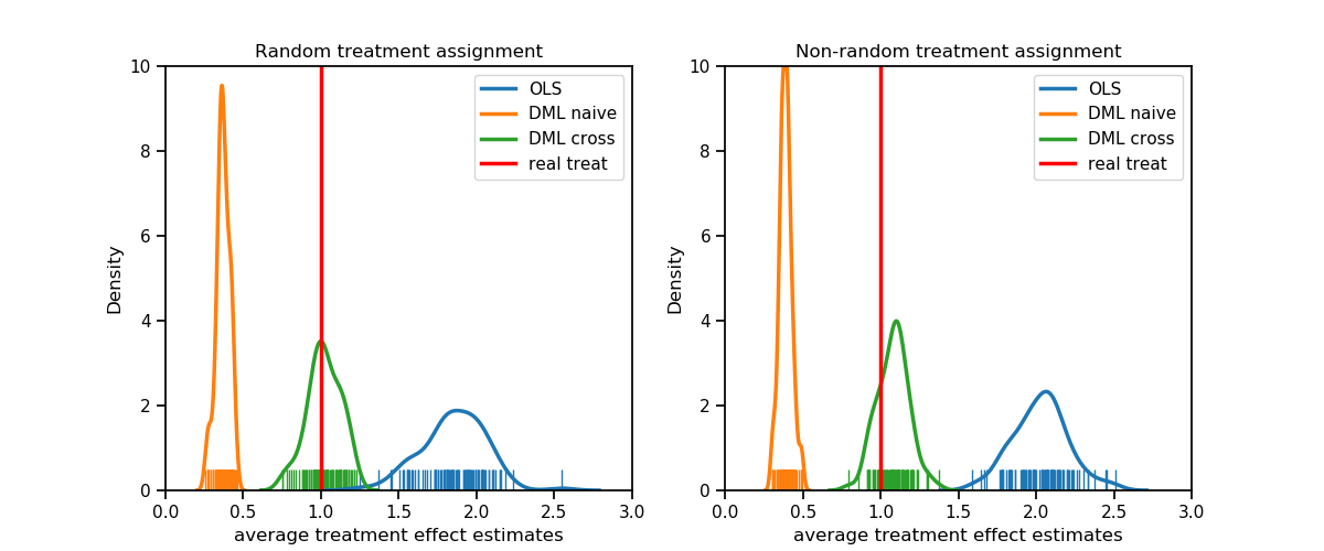
Both plots show that OLS as well as the naive estimator are obviously biased, while the bias of OLS is stronger. In the random assignment case the cross fit double machine learning estimator on the other side meets on average $\, \theta \,$ perfectly and even in the non-random assignment it is still close the the true value compared to the other two alternatives.
Discussion
This blog post has introduced a novel software that has the potential of supporting researchers from all fields in their model setup and evaluation.
Due to the ease of use, people without a mathematical or computer-scientific background will be able to apply its core functions, while others will be capable of refining the underlying principles.
Being entirely written in Python and hosted on Pypi and Github with a public license, the project is now accessible to the scientific community.
Based upon a thoroughly tested and often-used partial linear model, the exact relations between all variables are known and easily adjustable for personalized use.
Consequentially, our software provides a general toolset to fit and compare various models for all purposes.
A practical application has been presented in terms of Double Machine Learning, where a constant and known treatment effect was a parameter to be estimated.
The example displayed the performance of some naive and some sophisticated models and their capability of accurately predicting the parameter of interest under varying circumstances (random vs. non-random assignment).
References
Chernozhukov, Victor, Denis Chetverikov, Mert Demirer, Esther Duflo, Christian Hansen, and Whitney Newey. 2017. "Double/Debiased/Neyman Machine Learning of Treatment Effects." American Economic Review, 107 (5): 261-65. DOI: 10.1257/aer.p20171038
Dorie, Vincent & Hill, Jennifer & Shalit, Uri & Scott, Marc & Cervone, Dan. (2017). Automated versus Do-It-Yourself Methods for Causal Inference: Lessons Learned from a Data Analysis Competition. Statistical Science. 34. 10.1214/18-STS667.
Goldfeld, Keith (2019). simstudy: Simulation of Study Data. R package version 0.1.14. https://CRAN.R-project.org/package=simstudy
Jacob, D., Lessmann, S., & Härdle, W. K. (2018). Causal Inference using Machine Learning. An Evaluation of recent Methods through Simulations
Powers, S, Qian, J, Jung, K, al, et. Some methods for heterogeneous treatment effect estimation in high dimensions. Statistics in Medicine. 2018; 37: 1767– 1787. https://doi.org/10.1002/sim.7623
Robinson, P. M. (1988). Root-N-consistent semiparametric regression. Econometrica 56, 931–954
B. Rubin, Donald & John, L. (2011). Rubin Causal Model. 10.1007/978-3-642-04898-2_64.