Correcting for Self-selection in Product Rating: Causal Recommender Systems

Authors: Karolina Grubinska & Médéric Thomas

Table of Contents

1. An Introduction to Recommender Systems
2. [Motivation] (#motivation)
3. [Overview of Methods] (#methods)

• [Matrix Completion Problem] (#matrix)
• [Singular Value Decomposition] (#svd)

4. [Problem Definition] (#problem)

• [The Missing-at-Random Assumption] (#mar)
• [Does MAR really hold?] (#marhold)

5. [Our Goal in This Framework] (#goal)

• [In Mathematical Terms] (#maths)

6. [A proposal for Causal Recommender System: Causal Embeddings] (#cause)

• [Causal Setup] (#causal)
• [Results Comparison] (#results)

7. [Conclusions] (#conclusions)
8. [Bibliography] (#bibliography)

An Introduction to Recommender Systems

One of the main characteristics of a modern, digital society that we currently live in is the heterogeneity of available items. In the past few years, the extension of the online market surpassed the traditional retail (Bonner & Vasile, 2018), causing an evolution of business models. The customers now have access to an abundant number of resources, which is no longer limited by the size of a physical store and the companies needed to respond to those changes. Because no shop assistant would support the process of decision-making, new challenges arose together with easier access to goods and services. It created a need to implement Recommendation Systems (RS), that would leverage customers’ data to create personalized suggestions for products and identify relevant information for them. The basic idea in the functionality of such a system is to infer users’ preferences based on their historical data and then target the additional products that the customer will like.

Motivation

The application of the recommendation engine can not only make the process of decision-making more easy for the customers by providing them with personalized content. Following Bonner & Vasile (2018), product recommendation systems have become the key driver of demand on today’s’ market. Some recent research has shown that the most well-known e-commerce companies could increase their up-selling revenue from 10 to 50 percent by implementing Recommender Systems. In the case of Amazon, one of the leaders on the online market, roughly 35 percent of sales are driven by personalized product suggestions (McKinsey & Company, 2016). Furthermore, firms can have growth not only in sales but also in consumer’s usage. Continuous responding to customers preferences by providing them with personalized content increases the likelihood to stay loyal subscribers of firms’ service and strengthens the habits in their usage patterns and buying behavior.

The classical Recommendation Systems are based on the observational data which carry two types of information: the items that each user interacted with and their feedback on how much they enjoyed such an item (Liang, Charlin & Blei, 2016).

• In case of explicit feedback, a user can leave a high or low rating which indicates their satisfaction with the product. It can be expressed by giving for example a 1-5 star rating.
• In implicit feedback, the opinion of the client is expressed as a binary decision by either clicking, purchasing, viewing or simply ignoring a product. In contrast to the first option, implicit data is easier to obtain and does not require any effort from the side of the customers because it is the product of their natural browsing behavior.

However, the observed feedback requires interaction in the first place and therefore, it is the result of users preferences and product selection. Knowing this, the absence of some feedback carries useful insights that are the object of research in the field of causal inference. The causal framework in this context examines the influence of unobserved confounders. Those are some underlying factors that may affect both users’ exposure to products and their feedback about it. The recent research has shown that not taking this influence into account while generating recommendations is leading to biased conclusions about recommendation effect, meaning self-selection bias caused by the user or the actions of recommender system itself (Schnabel et al., 2017).

The aim of the following work is to present and measure the causal effect of recommendation. In the further sections, we will present to this extent an existing model, CausE, which was introduced by Bonner and Vasile (2018) as a strategy to leverage the classical recommendation approach. The two nodes of observational feedback explained above will require the introduction of some assumptions to present causal problem of recommendation in more detail.

Overview of Methods

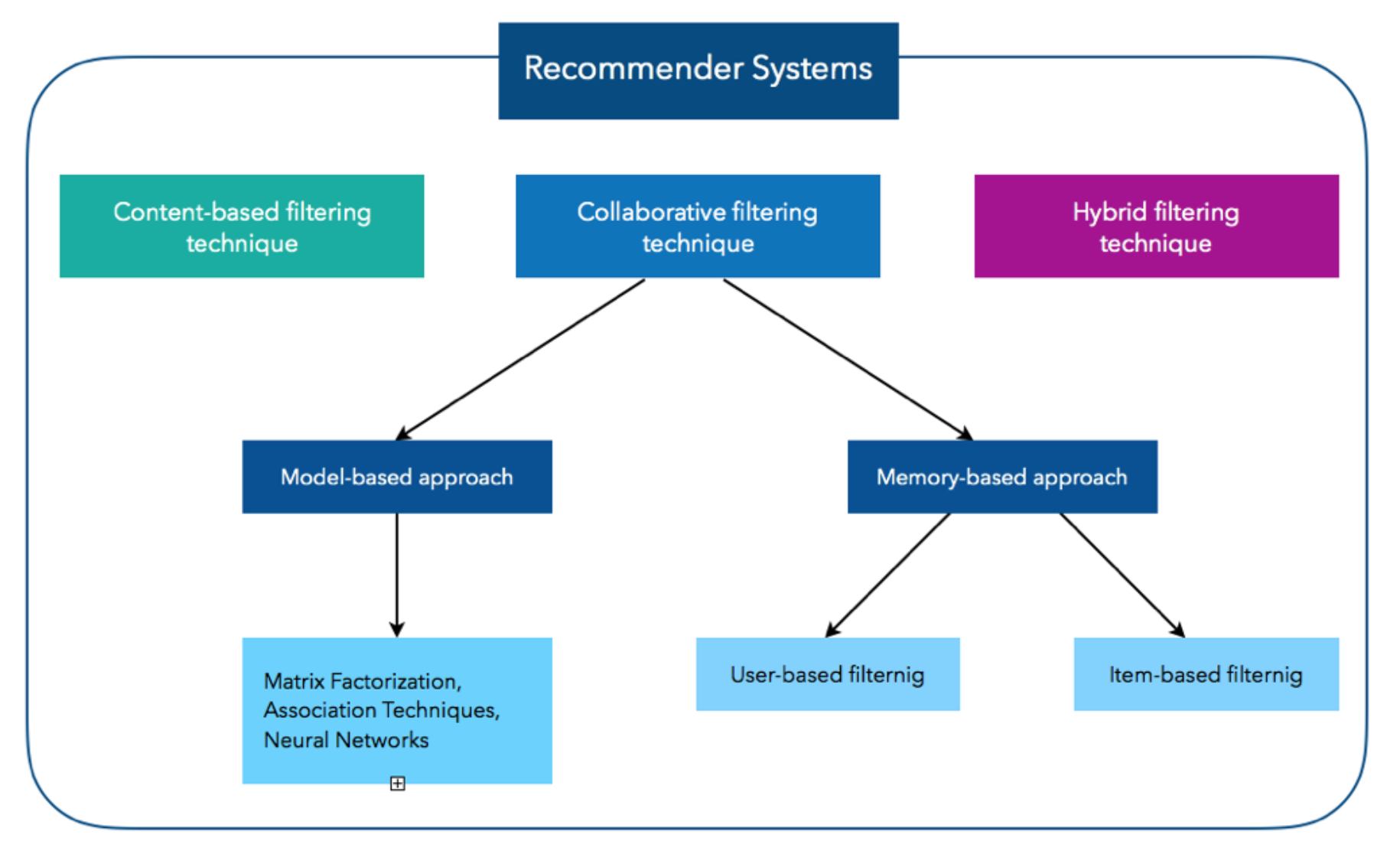
The graph above illustrates the three fundamental methods to build a Recommender System. The first method, Content-based filtering (CB) is based on users’ history. The idea of this approach is to create a profile for each user and all items with a description of its main characteristics. Then, the algorithm is choosing the most liked products and recommends to the user the item with the most similar content. Another approach is called Collaborative Filtering (CF) and it relies on past users’ behavior, meaning given ratings or clicked items without requiring the creation user and item’s profiles. It aims to identify new user-item associations by analyzing relationships between user and interdependencies among products. The two main areas of Collaborative Filtering are the Memory-based and Model-based Techniques. The first approach concentrates on the computation of relationships across products or items separately, while the Model-based approach is investigating both items and ratings by characterizing them. The last method is combining both of the techniques, CB and CF. In the following lines, we will concentrate on Collaborative Filtering, which can be globally thought as a matrix-completion problem (Koren, Bell & Volinsky, 2009).

Matrix Completion Problem

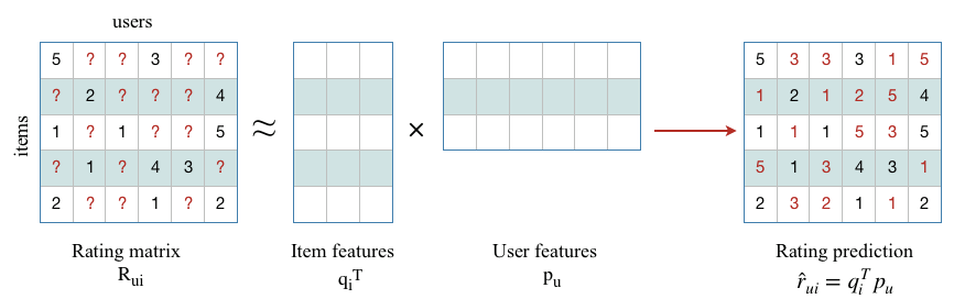
The matrix on the left side of the equation represents the initial setting that one has to face while preparing the data to apply a CF algorithm. In the rating matrix $R_{ui}$, the rows are representing items from the dataset and each column represents a user. The numbers inside the matrix are the ratings. Filling the empty cells that have been replaced by “?” symbol, can be seen as a matrix completion problem where one tries to estimate the missing numbers. This problem can be solved using a wide range of Matrix Factorization methods. The main idea behind those techniques is to describe both items and users by vectors of factors that would approximately replicate the initial user-item matrix after multiplication (Koren, Bell & Volinsky, 2009).

Singular Value Decomposition

Before we will introduce the causal framework for recommendation, in the notebook below we will present the application of Collaborative Filtering using Singular Value Decomposition algorithm as our benchmark model.

Problem Definition

The first goal of our Recommender System is to infer users’ preferences for an item and based on that, to predict the products that should be recommended. As mentioned in the chapter about our motivation, in the recommendation setting we face two types of information: about the interaction and click or rating. The traditional RS use the rating or click data alone to infer customers preferences. However, the implicit assumption behind models trained and evaluated only on the observed data is that the absence of some feedback carries no information, meaning the unobserved ratings or clicks are missing at random (MAR) (Kula, 2009). But are they really ?

The Missing-at-Random Assumption

Following the thoughts from the previous section, we want to investigate the validity of the MAR assumption on our dataset.

Our Data comes from the [Yahoo! R3 Dataset] (https://webscope.sandbox.yahoo.com/catalog.php?datatype=r&guccounter=1). It consists of explicit feedback by users, where one can directly observe how a user rates a song giving it 1-5 Stars. The songs from this dataset come from two different sources. The first source consists of ratings supplied by users during normal interaction with Yahoo! Music services and the other source consists of ratings for randomly selected songs collected during an online survey conducted by Yahoo! Research. Scaling this dataset provided us 157K ratings given by 1000 users and concerning 995 songs, coming only from the normal interaction scheme.

Does MAR really hold?

Following the [Kulas presentation] (https://resources.bibblio.org/hubfs/share/2018-01-24-RecSysLDN-Ravelin.pdf), if the ratings are randomly missing, the following has to hold:

How much a user likes a song will not influence the likelihood of leaving a rating.

As it can be seen in the graph above, users tend to leave more “1” (really dislike) or “5” (really like) ratings than the ratings in between. This is a clear evidence that a strong preference or aversion for a song by a user leads him to a higher probability of leaving a rating.

There are more sentences that could be derived from the MAR assumption, but this one should be enough to show the problematic behind it.

Ignoring the effect of unobserved ratings means ignoring some latent factors that influence the rating but also the probability that an item will receive a rating in the first place. Therefore, the assumption that the users consider each item independently at random does not hold in the reality and ratings are Missing Not at Random (MNAR). Consequently, the previously mentioned approach is biased by the exposure data.

Our Goal in This Framework

As Bonner and Vasile (2018) argued in their work, building a Recommender System should only aim to model customers’ preferences and to predict most suitable suggestions for new products. Many of the recent research works fall short to optimally model and measure the effect of influential nature of RS, meaning the change in users’ behaviour or their certain activity. We will follow these thoughts and steps to try to obtain the optimal treatment policy which aims to maximize the reward coming from each user with respect to the control recommendation policy. In other words, we want to maximize the Individual Treatment Effect (ITE). In our case, the control recommendation was the classical CF approach presented earlier, using Singular Value Decomposition with Stochastic Gradient Descent algorithm to solve the matrix completion problem.

In Mathematical Terms

To present learning recommendation policies as an optimization problem with respect to the Individual Treatment Effect requires the introduction of the following terms:

• $\Pi_x$ : stochastic policy, associating to each user $u_i$ and product $p_j$ a probability to be exposed to a recommendation
• $r_{ij} \sim r(.|u_i,p_j)$ : the true outcome/ reward for recommending product $p_{j}$ to user $u_i$
• $y_{ij} = r_{ij} \Pi_x(p_j | u_j)$ : the observed reward for the pair $i,j$ of user-product according to the logging policy $\Pi_x$
• The reward associated with a policy $\Pi_x$ : $$R^{\Pi_x} = \sum_{i,j}r_{ij}\Pi_x(p_j,u_j)p(u_i)$$
• The ITE value of of a policy $\Pi_x$ for a given user $i$ and a product $j$ defined as the difference between its reward and the control policy reward: $$ITE_{ij}^{\Pi_x} = R_{ij}^{\Pi_x} - R_{ij}^{\Pi_c}$$

We are interested in finding the policy $\Pi^*$ woth the highest sum of ITEs: $$\Pi^* = argmax_{\Pi_x} ITE^{\Pi_x}$$ where $$ITE^{\Pi_x}=\sum_{i,j}ITE_{ij}^{\Pi_x}$$

In order to find the optimal policy $\Pi^*$, we need to find for each user $u_i$, the product with the highest personalized reward $r_i^*$

In practice the reward $r_{ij}$ can not be directly observed but what we know about the observed reward $y_{ij}$ is that $y_{ij}$ $\sim$ $r_{ij}$$\Pi_x$$(p_j | u_j)$

With this knowledge, the unobserved reward $r_{ij}$ can be estimated using Inverse Propensity Scoring (IPS)-based methods: $$\hat{r_{ij}}\approx \frac{y_{ij}}{\Pi_c(p_j|u_i)}$$

However, one of the main critics about this approach lays in the fact, that in effect, the products with low probability under the logging policy $\Pi_c$ will receive higher estimated reward. But using simply uniform exposure would result in low quality of recommendation, because we usually don’t have large datasets about it, since many items come with only a few interactions.

The proposed solution is to use the biased data from the latest control policy and let the algorithm learn to predict the outcomes under under a randomized policy and use this transformation to rank the products by their estimated outcomes

The effect of this approach will be measured against the Matrix Factorization approach presented in the previous section

A Proposal for Causal Recommender System: Causal Embeddings

We based this part on the paper and code from Bonner & Vasile (2017), Causal Embeddings for Recommendation. [Source : https://arxiv.org/abs/1706.07639]

Causal Setup

We are interested in building a predictor for recommendation under random exposure of users to a song, because this is the way we can generate more value to the user by having a unbiased prediction model. As we said earlier, using a uniform exposure to recommendation ratings is resulting in low prediction quality, because we then have only a small portion of data, which would produce less stable estimators. In this framework, the authors have developed a way to use both randomized treatment exposure and control policy data together, to build a more robust predictor, which would still aim to maximize the sum of individual treatment effects.

To this extent, we are assuming the existence of two training samples :

• A very large group of interactions collected by exposure to the original control recommendation policy $c$.
• A smaller group of interactions collected with a fully uniform randomized policy $t$.

Those two samples are selected from the same group of users $U$. Our other - and principal - hypothesis is that the expected control and treatment rewards can be approximated as linear predictors over the shared user embedding representation.

Following the framework introduced in the above section, we want to approximate the Indivual Treatment Effect, in order to be able to maximize it in our Recommendation policy. From the latest hypothesis, we have :

$$\hat{ITE}_{i,j}=\langle p_j^t,u_i\rangle-\langle p_j^c,u_i\rangle$$

And by letting $W^{\delta}$ be the difference between $P^t$ and $P^c$, we can also have :

$$\hat{ITE}_{i,j}=\langle w_j^{\delta},u_i\rangle$$

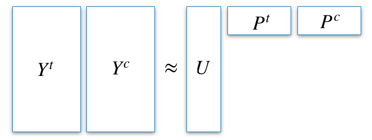
Our wish here is to recreate the embeddings matrices $U$, $P^t$ and $P^c$ in the most accurate way. To achieve this goal, we define a loss function $l$ to measure the difference between the approximated expected treatment reward $P^t$ and the observed one $Y^t$. Adding a penalization $\Omega$ on the weights, we have our final loss function for the uniformly-exposed dataset :

$$L^t=l(UP^t,Y^t)+\Omega(P^t)$$

Likewise, we can apply the same loss function to the control group of the dataset, in order to leverage it.

$$L^c=l(UP^c,Y^c)+\Omega(P^c)=l(U(P^t-W^{\delta}),Y^c)+\Omega(P^t,W^{\delta})$$

We want to minimize both loss functions, which can be seen as two different tasks. But they can also be merged into a single one, and by grouping them together, we have :

$$L_{CausE}^{Prod}=L(P^t,P^c)+\Omega_{disc}(P^t-P^c)+\Omega_{embed}(P^t,P^c)$$

Where :

• $L(.)$ is the reconstructed loss function with the concatenation matrix of $P^t$ and $P^c$.
• $\Omega_{disc}$ is a penalization function that weights the discrepancy between the two representations (treatment and control).
• $\Omega_{embed}$ is a penalization function that weights the embedding vectors.

We can also replace $P^c$ or $P^t$ by $W^{\delta}$ and have only one penalization function to include.

$$L_{CausE}^{Prod}=L(P^t,W^{\delta})+\Omega(W^{\delta})+\Omega (P^t)=L(P^t,W^{\delta})+\Omega_{embed}(P^t,W^{\delta})$$

The reason why the authors expected this algorithm to be more powerful and safer than a strict computation on a uniformly-exposed dataset, is that here the User embeddings are strengthened by the data we have on the original control policy. Therefore the embeddings that vary in this framework are only the Product ones, and the penalization on the difference between the two matrix representations should help to prevent any suspectful big change.

Results Comparison

Those conclusions are subject to the hyperparameters we entered. We have tried several combinations about it but we cannot guarantee that their optimization is perfect. More work would be needed to see how those results are influenced by the choices we made, such as the embedding size for example, or how the algorithms would react with a different dataset.

Conclusions

In the following project, we presented the current methods and approaches to build a Recommender System on Yahoo! R3 Dataset for songs recommendation. In the first part, we introduced Collaborative Filtering as our baseline method. We described a solution to this approach as the matrix factorization problem to evaluate the suggestions for a recommendation based on past users behavior and predict the missing entries in the user-item matrix. We used the classical Collaborative Filtering approach with the Singular Value Decomposition algorithm as our benchmark, noncausal model and optimized it using Stochastic Gradient Descent. Furthermore, we presented the limitations behind the MAR assumption on our dataset and how it leads to the presence of self-selection bias. In the main part, we followed the work of Bonner and Vasile (2018) and concentrated on the implementation of their approach to our dataset to obtain an unbiased predictor for recommendations. The proposed algorithm is an extension of matrix factorization which predicts the recommendation according to uniform exposure by learning from logged data containing outcomes from the biased recommendation policy. In the last section, we compared the performance of both models and it could be seen that the CausE algorithm outperformed the classical CF measured in both, ROC and RMSE metrics and with every parameter setup that has been tested. However, because the implementation of CausE required more steps and was more time costly a higher accuracy was expected. However, when it comes to deciding about the implementation of one of the models there is the tradeoff between complexity and efficiency, which is currently also one of the subjects of discussion in Data Science.

Bibliography

Bonner, S. & Vasile, F. (2018). Causal Embeddings for Recommendation. Proceedings of the 12th ACM Conference on Recommender Systems, pages 102-112.

Koren, Y., Bell, R. & Volinsky, C. (2009). Matrix Factorization Techniques for Recommender Systems. Computer, pages 30-37.

Liang, D., Charlin, L. & Blei, D. M. (2016). Causal Inference for Recommendation.

McKinsey & Company (2016). How retailers can keep up with consumers. [https://www.mckinsey.com/industries/retail/our-insights/how-retailers-can-keep-up-with-consumers]

Schnabel, T., Swaminathan, A., Singh, A., Chandak, N. & Joachims, T. (2016). Recommendations as Treatments: Debiasing Learning and Evaluation. Proceedings of Machine Learning Research (vol. 48), pages 1670-1679.