By Maximilian Kricke, Tim Peschenz | August 1, 2019
Applied Predictive Analytics Seminar - Causal KNN
Beyond estimating the overall effect of a treatment, the uplift, econometric and statistical literature have set their eyes on estimating the personal treatment effect for each individual. This blogpost highly relates to the paper of Hitsch & Misra (2018), where a novel, direct uplift modeling approach is introduced, called Causal KNN. The k-nearest neighbour algorithm provides an interesting opportunity for the estimation of treatment effects in small groups. To estimate the treatment effect, the Transformed Outcome, introduced by Athey and Imbens (2015b), is used. We will show that the Transformed Outcome is not only restricted to the Causal KNN modeling approach. Under several assumptions to the data, the Transformed Outcome equals in expectation to the true CATE. Hence it can be seen as a general tool for the parameter tuning in the context of Treatment Effect Analysis. Additionally, the Transformed Outcome can be used to evaluate different uplift models in terms of the MSE.
In the beginning, we will give a motivation for the topic, followed by an introduction of the methods presented by Hitsch & Misra (2018). In order to highlight the applicability of those methods, an implementation on real world data of a randomized E-Mail marketing campaign is given. We will perform the Causal KNN estimation as well as a Causal Tree estimation. In the end, the model performance is compared using MSE, AUUC and the Qini-Curve.
Motivation and Literature Foundation:
The analysis of causal effects is of high importance in many different areas. The testing of a new drug, the evaluation of a labor market program, or the optimization of a marketing campaign in a business setting are all influenced by an unobservable bias. Researchers in all these areas are facing the fundamental problem of causal inference, which is the fact that we never observe the individual treatment effect, but the outcome corresponding only to the assigned treatment. To grasp the concept of the Causal KNN the introduction of the potential outcome framework first given by Rubin (1974, 1977, 1978) is required: For every individual $i$ with the attributes $X_i$ in the population sample, we observe the outcome $Y_i(W_i)$ that corresponds to a specific treatment status $W_i=\text{{0,1}}$. For the given sample, the individual probability of receiving a treatment conditional on the individuals attributes is called the propensity score $P(W_i=1|X_i=x)=\mathbb{E}[W_i=1|X_i=x]=e(x)$ (Rosenbaum and Rubin, 1983). In this general framework, causal effects can be understood as comparisons of potential outcomes defined on the same unit.
This blogpost highly relates to the work “Heterogeneous Treatment Effect Estimation” of Hitsch & Misra (2018). Their work has a broad framework and deals with a variety of topics in the Treatment Effect Estimation especially in the business setting. In the first part, they are presenting an approach to compare several different targeting policies by using only one single randomized sample. They propose an inverse probability weighted estimator which is unbiased, qualitatively equivalent to a field experiment and cost effective. Maximizing the profit of a marketing campaign comes down to the knowledge of the Conditional Average Treatment Effect (CATE) $${\tau(x)}={\tau(x)}^{CATE}=\mathbb{E}[Y_i(1)-Y_i(0) | X_i=x]$$ As it follows from the fundamental problem of causal inference, the true CATE is not observable in general. Therefore the main part of their work is devoted to identification methods for the true CATE. They introduce three crucial assumptions to the data, to make the CATE identifiable.
Unconfoundedness:
$Y_i(0), Y_i(1) \bot W_i | X_i$.
It means, that ones individuals outcome does not depend on the treatment conditional on the covariates (Rubin, 1990). ‘The treatment assignment is random within a subset of customers with identical features’ (Hitsch & Misra, 2018). This condition can be fulfilled by using a randomized sample set. In marketing, it is often possible to address campaigns randomized, therefore this condition should be satisfied in general and especially in our application. We will see that this assumption is crucial for the derivation of an unbiased estimator for the CATE.
The Overlap Assumption:
$0 < e(x) < 1$
For general application, the propensity score has to be defined strictly between zero and one. If this assumption is violated, there would be no treated or untreated observation for specific values of the feature vector $X_i$. We will see that this assumption is also required to derive an estimator for the CATE.
Stable Unit Treatment Value Assumption (SUTVA):
The treatment received by customer i, $W_i$, has no impact on the behaviour of any other customer. There are no social interaction or equilibrium effects among the observed units. According to Hitsch and Misra, the SUTVA assumption should be satisfied in general marketing applications. It appears implausible to observe economically significant social effects, e.g. word-of-mouth, due to the receipt of a newsletter.
If those three assumptions are satisfied, we can calculate the true CATE by taking the mean difference between the outcome of treated and untreated units with identical features:
$\tau(x) = \mathbb{E}[Y_i|X_i,W_i = 1] - \mathbb{E}[Y_i|X_i,W_i = 0]$
It is unrealistic to assume that there are more than one customer with exactly the same feature set, especially for high dimensional data. And therefore the true CATE as given in the above formula needs to be estimated. Hitsch and Misra are presenting methods to predict the CATE indirectly via the outcome variable, i.e. $\mathbb{E}[(Y_i-\hat{\mu}(X_i,W_i))^2]$ (OLS, Lasso, Logit, Non-parametric models) as well as directly via the treatment effect, i.e. $\mathbb{E}[(\tau(X_i)-\hat{\tau}(X_i))^2]$ (Causal KNN, Treatment Effect Projection, Causal Forest). The aim of this blogpost is to explain and apply the Causal KNN estimation method that directly predict the individual incremental effect of targeting. Hitsch and Misra (2018) describe the indirect approaches as conceptually wrong in the field of uplift estimation. They recommend the usage of direct estimation methods, since they yield a more accurate estimation of the treatment effect.
To illustrate the proposed Causal KNN method to estimate the causal effects, we will utilize a business framework. Imagine: A company runs a marketing campaign. Now this campaign can consist of various customer treatments, such as a targeted price, a coupon or a newsletter. But how do you evaluate the campaigns’ success? At this point, Hitsch & Misra (2018) elaborate the dependency of marketing success from the individual targeting effort cost. A customer should be targeted if the individual profit contribution is greater than the targeting cost for this individual. It is shown that the CATE on an individual basis is sufficient to construct an optimal targeting policy. To then conduct a profit evaluation, the individual costs and margins are required, which are generally known for a company, but unknown in our data. Therefore, we will focus on estimating the causal effects without including the individual targeting costs by using Causal KNN in combination with the Transformed Outcome approach. In the business framework, the expected causal effects can be described through the CATE, which represents the incremental targeting effort effect.
Estimating ${\tau}(x)$ directly via Causal KNN regression
As mentioned before, the true CATE is not observable. Hitsch and Misra use a method to approximate the actual treatment effect via the Causal KNN regression. This approach allows to derive an estimator of the CATE on an individual unit level. The Causal KNN regression method is represented in the following equation:
where $Y_i$ represents the outcome values of the target variable and $N_K(x,0)$ and $N_K(x,1)$ denote the nearest neighbour units with treatment status $W_i = 1$ and $W_i = 0$ respectively. Since the Causal KNN algorithm takes the number of nearest neighbours $K$ as a freely selectable parameter, it is necessary to find a way to choose the optimal $K$ value. In order to present the real data implementation of the Causal KNN regression, the used data will be presented in the following.
Data Presentation
For the application of the presented methodology, data from an E-Mail targeting campaign was used, including 64,000 observations. The data entries represent customer transactions with serveral corresponding variables. The treatment variable “segment” originally includes three possible values, E-Mail for Women, E-Mail for Men and No E-Mail. There are three different target variables. “Visit” as the visitation of the companies website and “Conversion” of the customer are binary variables. The numeric variable “Spend” represents the amount of money spend by a customer in the following two weeks after the campaign. There are various covariates that characterize customers according to their personal properties and purchasing behaviour. The “Recency” represents the month since the last purchase was made. “History” and “History_Segment” include information about the amount of money spend in the last year, in dollars. “Mens” and “Womens” are binary variables that indicate whether a customer bought products for men or for women. The “Zip_Code” includes geographical information, grouped into Urban, Suburban and Rural regions. “Newbie” states whether a person was registered as a new customer in the past 12 month and the Channel represents on which ways a customer placed orders, i.e. via phone, mail or both. To provide a comprehensive overview about the data, an example table is presented, including first observations of the data set.
head(data)
| recency | history_segment | history | mens | womens | zip_code | newbie | channel | segment | visit | conversion | spend | idx | treatment |
|---|---|---|---|---|---|---|---|---|---|---|---|---|---|
| 10 | 2) 100-100-200 | 142.44 | 1 | 0 | Surburban | 0 | Phone | Womens E-Mail | 0 | 0 | 0 | 1 | 1 |
| 6 | 3) 200-200-350 | 329.08 | 1 | 1 | Rural | 1 | Web | No E-Mail | 0 | 0 | 0 | 2 | 0 |
| 7 | 2) 100-100-200 | 180.65 | 0 | 1 | Surburban | 1 | Web | Womens E-Mail | 0 | 0 | 0 | 3 | 1 |
| 9 | 5) 500-500-750 | 675.83 | 1 | 0 | Rural | 1 | Web | Mens E-Mail | 0 | 0 | 0 | 4 | 1 |
| 2 | 1) 0-0-100 | 45.34 | 1 | 0 | Urban | 0 | Web | Womens E-Mail | 0 | 0 | 0 | 5 | 1 |
| 6 | 2) 100-100-200 | 134.83 | 0 | 1 | Surburban | 0 | Phone | Womens E-Mail | 1 | 0 | 0 | 6 | 1 |
Data Preparation
After importing the e-mail data set, the non-numeric variables are converted into factors. Afterwards, all columns are examined with regard to missing values. There are no missing observations in the data set. Therefore, an imputation of missing values is not necessary for none of the variables.
To label the different observations in the data set, an index column was added, in order to be able to reassign all observations in the later steps of the analysis. The original data set contains three outcomes for the treatment variable, i.e. E-Mail for Women, E-Mail for Men and no E-Mail. Since the analysis is designed to deal with binary treatment variables, the three possible treatment values are reduced to either receiving an E-Mail or not. For the further process of the analysis, the binary variable “treatment” indicates solely whether units received a treatment. There is no distinction anymore between E-Mails for Women and Men.
Since the different treatments were randomly assigned with the same probability, the aggregation of the treatment yields at a propensity score of 2/3 for each individual. Therefore, the treatment assignment in the data set is slightly unbalanced. Since the difference between the number of treated and untreated customers is not too high, the unbalancedness should not cause any problems for the proposed method. For extremely unbalanced data sets with regard to the treatment status, the Causal KNN algorithm might not work, because it can become impossible to find sufficiently much treated or untreated nearest neighbours.
The KNN algorithm identifies the nearest neighbours of an individual $i$ by calculating the euclidean distances between target variable outcomes of different units. Therefore, the method can only deal with numeric variables. To meet this requirement, the non-numeric covariates are Transformed into dummy variables, using the mlr package.
Causal KNN Implementation
In the application here, the propensity score is the probability of receiving an email, i.e. the ‘targeting probability’ for each unit. The targeting probability is constant over all customers with a value of 2/3 in our application. That means, a randomly choosen customer receives an email with a probability of 2/3.
The algorithm starts with selecting the k treated and untreated nearest neighbours for each observation. The nearest neighbours are selected based on the covariates, using the euclidean distance measure on the standardized data. However, every other distance measure would be similarily feasible, depending on the application framework. Afterwards, the individual treatemnt effects are derived by computing the differences between the mean outcome values of the treated and the untreated nearest neighbours for all units. This yields at an estimation of the CATE for each observation in the data set. A brief description of the algorithm is given by the following figure:
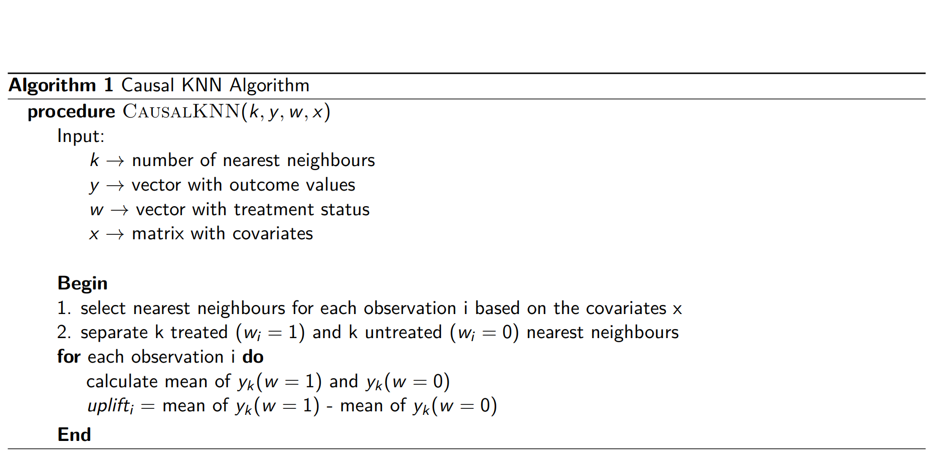
The Causal KNN alorithm starts with selecting the k treated and untreated nearest neighbour observations for each unit i. To allow for a simple selection of both groups, the data set is separated into two data frames, containing the treated and untreated observations respectively.
#select data partition for training
data_d = data_[1:25000, ]

###splitting data set
#1 no treatment
data_nt = data_d[which(data_d$segment.No.E.Mail == 1),]

#2 treatment
data_t = data_d[which(data_d$segment.No.E.Mail == 0),]
The KNN search is done by using the FNN package in R. This package allows to extract the index values of the nearest neighbours for each observation and the corresponding distances. An important aspect of Causal KNN is to find the optimal value of $K$ for a specific application setting. To check for several values of k, it is necessary to specify the maximum number of nearest neighbours, that should be tested. The maximum possible value of $K$ is restricted by the minimum total number of treated or untreated observations, i.e. the minimum number of rows of the data frames with the two treatment groups.
A very useful feature of the FNN package is the possibility to specify different data sets for the search space and the observations for which nearest neighbours have to be found. This allows to conduct a simple search for nearest neighbours among the treated and untreated observations. There are two data frames resulting from both steps of the search process. The “treated_nn” data frame includes the nearest neighbours with treatment status $W_i=1$ and “untreated_nn” those with treatment status $W_i=0$. These two data sets build the basis for the next step of the algorithm, i.e. the identification of the optimal value of $K$.
###Causal KNN
#install.packages("FNN")
library(FNN)

#setting parameter k for the maximum number of nearest neighbours to test for
k = 3000
k = k + 1

#select columns to be eliminated for nearest neighbour search
drop_cols = c("visit",
              "spend",
              "conversion",
              "idx",
              "treatment",
              "segment.Mens.E.Mail",
              "segment.Womens.E.Mail",
              "segment.No.E.Mail")

#garbage collection to maximize available main memory
gc()

#calculate indices of k treated nearest neighbours
treated_nn = get.knnx(data_t[, !(names(data_t) %in% drop_cols)],
                      query = data_d[, !(names(data_d) %in% drop_cols)],
                      k = k)
treated_nn = data.frame(treated_nn$nn.index)

#deleting first column
treated_nn = treated_nn[, 2:ncol(treated_nn)]


#calculate indices of k untreated nearest neighbours
untreated_nn = get.knnx(data_nt[, !(names(data_nt) %in% drop_cols)],
                        query = data_d[, !(names(data_d) %in% drop_cols)],
                        k = k)
untreated_nn = data.frame(untreated_nn$nn.index)

#deleting first column
untreated_nn = untreated_nn[, 2:ncol(untreated_nn)]


#replacing index values
treated_nn = sapply(treated_nn, FUN = function(x){
  data_t$idx[x]
})

untreated_nn = sapply(untreated_nn, FUN = function(x){
  data_nt$idx[x]
})
Comparison of Causal KNN and the Two-Model-Approach
At this point, a distinction between the Causal KNN and the Two-Model-Approach has to be made, since both methods seem to be similar. According to Rzepakowski and Jaroszewicz (2012, 2), the idea behind the two model approach is to build two separate models, to estimate the treatment effect. One Model is trained, using the treatment, and the other one using the control data set. After building the two models, the treatment effect estimations are calculated by subtracting the predicted class probabilities of the control model from those of the treatment model. This yields at a direct estimation of the difference in the outcome, caused by the treatment. An advantage of the two model approach is that it can be applied with any classification model (Rzepakowski and Jaroszewicz, 2012). A possible problem that might arise with this approach, is that the uplift might be different from the class distributions. In this case, the both models focus on predicting the class, rather than the treatment effect. The Causal KNN Algorithm also calculates the difference between the predicted outcomes of the treated and untreated observations in a data set. The number of observations that are taken into account, is limited by the KNN parameter $K$. Therefore, the Causal KNN algorithm itself can be possibly seen as a special case of the two model approach. An important aspect of the described method here, is the usage of the Transformed Outcome for the tuning of the Causal KNN model. Since the combination of Causal KNN and the Transformed Outcome allows to calculate the CATE estimations directly, it is not appropriate to completely assign this to the group of two model approaches. According to Rzepakowski and Jaroszewicz (2012, 2), the two model approach is different from the direct estimation methods, since it focuses on predicting the outcome of the target variable to estimate the treatment effect, rather than predicting the treatment effect itself. As already shown above, the Causal KNN algorithm should be rather categorized as a direct estimation approach (Hitsch and Misra, 2018) and should therefore not be seen as a pure two model approach.
To estimate a robust CATE, we would likely use all customers in the neighborhood. A high value for K increases the accounted neighborhood, while it decreases the similarity between the customers. Therefore, the estimation depends on the choice of K. To find an optimal value of K, we want to minimize the squared difference between $\hat{\tau}_K(x)$ and the Transformed Outcome $Y^*$. This is called the Transformed Outcome Approach, which will be described in the following.
Transformed Outcome Approach
Naturally, the optimal value of $K$ is given for the minimum of the Transformed Outcome loss:
$\mathbb{E}[(\tau_k(X_i)-\widehat{\tau_k}(X_i))^2]$
Unfortunately, as mentioned before, this criterion is infeasible, since the true CATE $\tau_K(X_i)$ is not observable. The Transformed Outcome approach is a method to somehow overcome the described fundamental problem of Causal inference by estimating the true CATE. In the literature, we find multiple approaches to do so. Gutierrez (2017) presents three different methods. First,he mentions the two-model approach that trains two models, one for the treatment group and one for the control group. Second, he mentions the class transformation method that was first introduced by Jaskowski and Jaroszewicz (2012). Their approach works for binary outcome variables (i.e. $Y_i^{obs.}=\text{{0,1}}$) and a balanced dataset (i.e. $e(X_i)=\frac{1}{2}$). A general formulation for the class transformation, which is even applicable for numeric outcome variables and an unbalanced dataset is given by Athey and Imbens (2015b). The Transformed Outcome is defined as follows:
$Y_i^*=W_i\cdot\frac{Y_i(1)}{e(X_i)}-(1-W_i)\cdot\frac{Y_i(0)}{1-e(X_i)}$
We can rewrite this formula:
$Y_i^*=\frac{W_i - e(X_i)}{e(X_i)(1-e(X_i))}\cdot Y_i^{obs.}$
The latter formula allows us to calculate the Transformed Outcome with the observed outcome. In case the propensity score is constant for every individual, i.e. complete randomization, the formula simplifies to $Y_i^*=Y_i^{obs}/e(x)$ for the treated individuals and $-Y_i^{obs}/(1-e(x))$ for the individuals that were not treated (c.f. Athey and Imbens 2015b).
Now, why is the Transformed Outcome helpful? In the following, we will present two appealing properties of the Transformed Outcome.
First, with the required assumption of unconfoundedness and no overlap, it can be shown that the Transformed Outcome is an unbiased estimator for the CATE:
$Y_i^*=W_i\cdot\frac{Y_i(1)}{e(X_i)}-(1-W_i)\cdot\frac{Y_i(0)}{1-e(X_i)}\quad|\quad\mathbb{E}[\cdot|W_i,X_i=x]$
$\Longrightarrow\mathbb{E}[Y_i^*]=\mathbb{E}[W_i|X_i=x]\cdot\frac{\mathbb{E}[Y_i|W_i=1,X_i=x]}{e(X_i)}-\mathbb{E}[1-W_i|X_i=x]\cdot\frac{\mathbb{E}[Y_i|W_i=0,X_i=x]}{1-e(X_i)}$
$=e(X_i)\cdot\frac{\mathbb{E}[Y_i|W_i=1,X_i=x]}{e(X_i)}-(1-e(X_i))\cdot\frac{\mathbb{E}[Y_i|W_i=0,X_i=x]}{1-e(X_i)}$
$=\mathbb{E}[Y_i|W_i=1,X_i=x]-\mathbb{E}[Y_i|W_i=0,X_i=x]\quad|\quad\textbf{Unconfoundedness: $Y_i(0), Y_i(1) \bot W_i | X_i$ }$
$=\mathbb{E}[Y_i(1)-Y_i(0)|X_i=x]$
$=\tau(X)$
If the overlap assumption is violated, it would not be possible to determine $\mathbb{E}[Y_i|W_i=1, X_i=x]$ and $\mathbb{E}[Y_i|W_i=0, X_i=x]$, because there would be only treated or untreated individuals for specific values of $x$. Since the estimator $Y_i^*=\tau_K(X_i)+\nu_i$ is unbiased, the error term $\nu_i$ is orthogonal to any function of $X_i$ (i.e. exogeneity assumption $\mathbb{E}[\nu_i|X_i]=0$).
The second appealing property of the Transformed Outcome is then demonstrated by Hitsch and Misra (2018):
$\mathbb{E}[(Y_i^*-\widehat{\tau_K}(X_i))^2|X_i] = \mathbb{E}[({\tau_K}(X_i)+\nu_i-\widehat{\tau_K}(X_i))^2|X_i]$
$=\mathbb{E}[({\tau_K}(X_i)-\widehat{\tau_K}(X_i))^2+2\cdot({\tau_K}(X_i)-\widehat{\tau_K}(X_i))\cdot\nu_i+\nu_i^2|X_i]$
$=\mathbb{E}[({\tau_K}(X_i)-\widehat{\tau_K}(X_i))^2|X_i]+\mathbb{E}[\nu_i^2|X_i]$.
$\Longrightarrow\mathbb{E}[(Y_i^*-\widehat{\tau_K}(X_i))^2]=\mathbb{E}[({\tau_K}(X_i)+\nu_i-\widehat{\tau_K}(X_i))^2)]=\mathbb{E}[({\tau_K}(X_i)-\widehat{\tau_K}(X_i))^2]+\mathbb{E}[\nu_i^2]$
In equation three we used the exogeneity assumption as well as the linearity of the expected value operator. As we can see, $\mathbb{E}[\nu_i^2]$ does not depend on the value of K, so minimization of the Transformed Outcome loss also minimizes the infeasible outcome loss. Therefore the Transformed Outcome allows us to estimate the true CATE and with this, we can find an optimal value for the parameter k.
Parameter Tuning using the Transformed Outcome
An essential part of the Causal KNN algorithm is the parameter tuning to specify the value of $K$, that leads to the most accurate treatment effect estimations. For the parameter tuning, several values for $K$ are tested and different CATE estimations are stored in a separate data frame. To derive estimations for all observations in the data set, the differences of the mean outcome variable values, of the $K$ treated and untreated nearest neigbours, are calculated. Repeated iterations of this procedure yields a data frame, containing the individual uplift estimations for different values of $K$. To select the most accurate estimation, the Transformed Outcome is used to decide for a preferable $K$ value.
###parameter tuning to find optimal k value
#setting parameters for the number of neigbours
k_start = 50
k_end   = 3000
steps   = 50

#creating sequence of k values to test for
k_values = seq(from = k_start, to = k_end, by = steps)

#preparing uplift data frame
uplift = data.frame("idx" = data_d$idx,
                    "treatment" = data_d$treatment)

#calculating uplift for specified k values
for (k in k_values) {
  reaction_nt = apply(untreated_nn, MARGIN = 2,
                      FUN = function(x){
                        mean(data_d$visit[x[1:k]])
                      }
  )

  reaction_t = apply(treated_nn, MARGIN = 2,
                     FUN = function(x){
                       mean(data_d$visit[x[1:k]])
                     }
  )

  uplift[paste("uplift_",k, sep = "")] = reaction_t - reaction_nt

  print(paste("k = ", k))
}
Transformed Outcome Loss Calculation
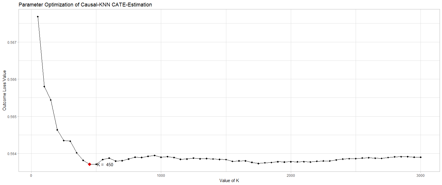
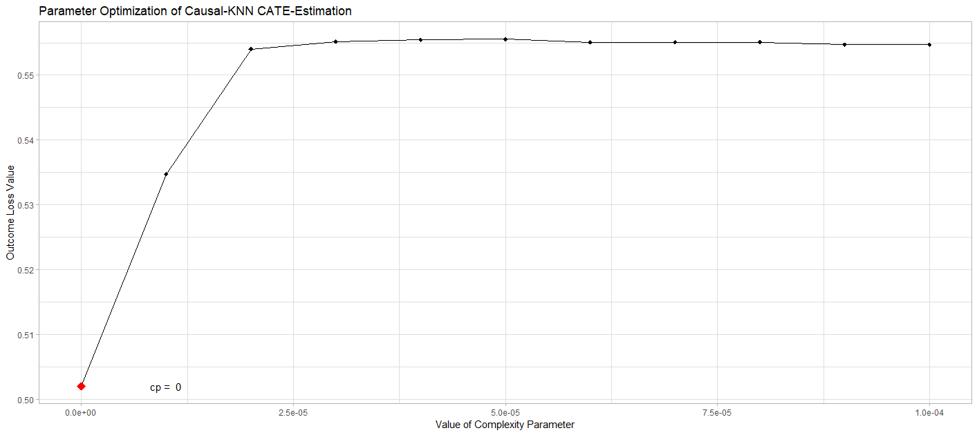
After calculating the various uplift estimations by varying the tuning parameter $K$ the Transformed Outcome as a proxy for the true CATE, is constructed. The calculation of the Transformed Outcome requires the knowledge of the propensity score, the treatment status and the original value of the target variable as inputs. By using the formula introduced above, the Transformed Outcome can be easily calculated for the actual target variabe visit. To decide on a value of $K$, the Transformed Outcome loss is calculated for each potential $K$ value by computing the mean squared difference between the Transformed Outcome and the various treatment effect estimations. The estimation, that yields at the minimal value of the Transformed Outcome loss, indicates the most accurate value for $K$, as shown by Hitsch and Misra (2018). The following plot was created to depict the development of the outcome loss with varying values of $K$. When increasing the number of nearest neighbours that are taken into consideration, the accuracy of the CATE estimation increases in the beginning. However, when increasing $K$ over a certain level, the heterogeniety among the nearest neighbours increases too much. That leads to less accurate estimations of the treatment effects. Therefore the aim is to find an optimal number of nearest neighbours, where sufficiently observations are taken into account, without increasing the heterogeniety too much.
###Transformed Outcome

#Identify/Set the propensity score

e_x = mean(data_d$treatment)

#function for Transformed Outcome
Transformed_outcome = function(e_x, w_i, target){
  return(((w_i - e_x)/(e_x*(1-e_x)))*target)
}

#apply function on all observations
trans_out = sapply(uplift$idx, FUN = function(x){
  Transformed_outcome(e_x = e_x,
                      w_i = data$treatment[x],
                      target = data$visit[x])
})

uplift$trans_out = trans_out

#Transformed Outcome loss
outcome_loss = data.frame("k" = k_values, "loss" = 0)

#find optimal k value from Transformed Outcome loss
for (i in 1:length(k_values)){
  outcome_loss[i, 2] = mean((uplift$trans_out -
                               uplift[, i + 2])^2)
}

#find minimal outcome loss value
outcome_loss$k[which.min(outcome_loss$loss)]
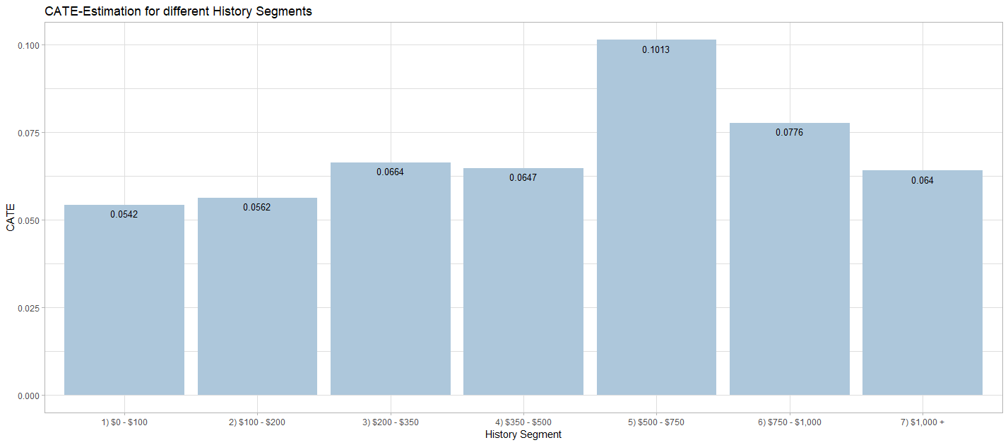
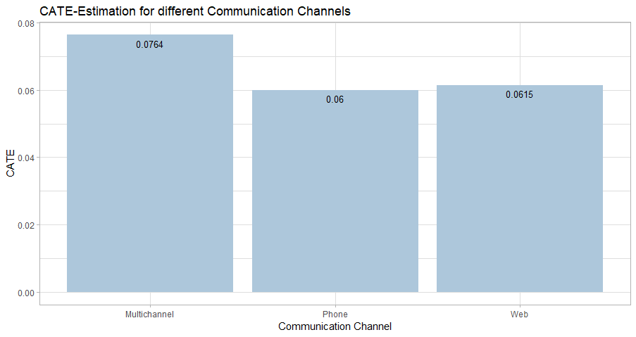
After finding the most accurate estimation of the CATE, it is possible to extract valuable insights from the data. This information can be used to plan targeting policies for future campaigns. Since the Causal KNN algorithm delivers treatment effect estimation on an individual level, it is easily possible to extract several other treatemnt effect measures. Furthermore, different CATE estimations based on different dimensions of the data can be calculated by grouping the observations.
Another advantage of the Causal KNN method is the high flexibility with regard to the target variable. As already shown, the algorithm works with binary outcome variables, i.e. visit in this case. By simply exchanging the target variable with a numeric one (“spend”), the algorithm can be executed similarily, without further modifications to the code. The CATE estimations represent an approximation of the total uplift, that is expected in the case of a treatment. Therefore, the CATE for the target variable “spend” indicates the expected absolute increase or deacrease of spendings for each individual, when a treatment is assigned. The application of the Causal KNN algorithm for numeric target variables does not need further changes to the implementation, instead of changing the outcome variable from visit to spend. Therefore, the code is not provided here in the blogpost. A possible implementation can be seen here: (https://github.com/mkrcke/APA/blob/master/src/07_causal_knn_numeric.R). Although the data theoretically allows for an estimation of the CATE for the variable “spend”, the insights of that estimation are not that valuable, because the dataset is extremely unbalanced with regard to the actual conversions (i.e. “spend” $> 0$).
Causal KNN for optimal Targeting Policy Prediction
The next section deals with the Causal KNN method in an application case, where a targeting policy has to be developed, based on the CATE estimations. From the model training and parameter tuning of previous steps, it was possible to find a best fitting value for the $K$ nearest neighbours that are taken into account. This value is now used in the prediction setting, where we assume that we do not know the actual outcome value.
The aim is to find those individuals, where a treatment increases the value of the outcome variable the most. By specifying a fixed percentage of the population, we are able to select the most profitable individuals for a treatment assignment. For the test data, we assume that we did not decide for a treatment assignment yet and do not have any information about the individual outcome values. Therefore, we are not able to calculate the Transformed Outcome for the test data set. Since we already estimated optimal parameter of k, we use this value here as parameter for the Causal KNN algorithm. The difference is now that we do not search for treated and untreated nearest neighbours in the test data set. We are not able to do so, because we did not decide for any treatment assignment yet. We rather search the neighbours for the observations in the training data, which we already used for finding the optimal k value.
test_set = createDummyFeatures(data[25001:30000, ])
test_set$idx = 1:nrow(test_set)

#splitting data set
#1 no treatment
data_nt = data_d[which(data_d$segment.No.E.Mail == 1),]

#2 treatment
data_t = data_d[which(data_d$segment.No.E.Mail == 0),]


#running Causal KNN for test set to calculate MSE
#select target columns
drop_cols = c("visit",
              "spend",
              "conversion",
              "idx",
              "treatment",
              "segment.Mens.E.Mail",
              "segment.Womens.E.Mail",
              "segment.No.E.Mail",
              "uplift")

#setting optimal k value from the parameter tuning above
k = outcome_loss$k[which.min(outcome_loss$loss)] + 1


#calculate indices of k treated nearest neighbours
treated_nn = get.knnx(data_t[, !(names(data_t) %in% drop_cols)],
                      query = test_set[, !(names(test_set) %in% drop_cols)],
                      k = k)
treated_nn = data.frame(treated_nn$nn.index)

#deleting first column
treated_nn = treated_nn[, 2:ncol(treated_nn)]


#calculate indices of k untreated nearest neighbours
untreated_nn = get.knnx(data_nt[, !(names(data_nt) %in% drop_cols)],
                        query = test_set[, !(names(test_set) %in% drop_cols)],
                        k = k)
untreated_nn = data.frame(untreated_nn$nn.index)

#deleting first column
untreated_nn = untreated_nn[, 2:ncol(untreated_nn)]

#replacing index values
treated_nn = sapply(treated_nn, FUN = function(x){
  data_t$idx[x]
})

untreated_nn = sapply(untreated_nn, FUN = function(x){
  data_nt$idx[x]
})

#transpose data frames
treated_nn = t(treated_nn)
untreated_nn = t(untreated_nn)

#preparing uplift data frame
uplift = data.frame("idx" = test_set$idx,
                    "treatment" = test_set$treatment)

reaction_nt = apply(untreated_nn, MARGIN = 2, FUN = function(x){
  mean(data_d$visit[x[1:k-1]])
})

reaction_t = apply(treated_nn, MARGIN = 2, FUN = function(x){
  mean(data_d$visit[x[1:k-1]])
})

uplift[paste("uplift_", k, sep = "")] = reaction_t - reaction_nt
Application of Transformed Outcome Approach for general Uplift Models
Causal Tree Model
The parameter tuning using the Transformed Outcome loss is equally useful for other uplift applications. To show this, the same methodology that was applied to determine the optimal $K$ value for the Causal KNN model, is used here to find optimal parameters for a causal tree. Different values for parameters are tested and evaluated by using the Transformed Outcome loss. Again, the minimal outcome loss value indicates the most favorable parameter value for the model estimation.
#using Transformed Outcome for tuning parameters of other uplift models
#different cp for causal tree

#install.packages("devtools")
#library(devtools)
#install_github("susanathey/causalTree")

library(causalTree)

#setting parameters for the complexity parameters to test for
cp_start = 0
cp_end = 0.0001
cp_steps = 0.00001

#creating sequence of k values to test for
cp_values = seq(from = cp_start, to = cp_end, by = cp_steps)
length(cp_values)

uplift_ct = data.frame("idx" = data_d$idx, "treatment" = data_d$treatment, "visit" = data_d$visit)

#calculating uplift for specified min size values
for (cp in cp_values) {
  causal_tree = causalTree(visit~.-spend -conversion -idx -segment.Mens.E.Mail -segment.Womens.E.Mail -segment.No.E.Mail, data = data_d, treatment = data_d$treatment, split.Rule = "CT", cv.option = "CT", split.Honest = T, cv.Honest = T, split.Bucket = F, xval = 5, cp = cp, propensity = e_x)

  uplift_ct[paste("uplift_",cp, sep = "")] = sapply(causal_tree$where, FUN = function(x){causal_tree$frame$yval[x]})

  print(paste("cp =", cp))
}


#calculate the Transformed Outcome
trans_out_ct = sapply(uplift_ct$idx, FUN = function(x){
  Transformed_outcome(e_x = e_x, w_i = data_d$treatment[x], target = data_d$visit[x])
})

uplift_ct$trans_out_ct = trans_out_ct

#Transformed Outcome loss
outcome_loss_ct = data.frame("cp" = cp_values, "loss" = 0)

#find optimal cp value

for (i in 1:length(cp_values)){
  outcome_loss_ct[i, 2] = mean((uplift_ct$trans_out_ct - uplift_ct[, i+3 ])^2, na.rm = TRUE)
}

outcome_loss_ct

#find minimal value
min(outcome_loss_ct$loss)

outcome_loss_ct$cp[which.min(outcome_loss_ct$loss)]

plot(outcome_loss_ct$loss)

cp_plot = ggplot(data = outcome_loss_ct) +
  geom_line(aes(x = outcome_loss_ct$cp, y = outcome_loss_ct$loss)) +
  geom_point(aes(x = outcome_loss_ct$cp, y = outcome_loss_ct$loss), size=2, shape=18) +
  geom_point(aes(x = outcome_loss_ct$cp[which.min(outcome_loss_ct$loss)], y = min(outcome_loss_ct$loss)),
             size = 4, shape = 18, color = "red") +
  geom_text(aes(x = outcome_loss_ct$cp[which.min(outcome_loss_ct$loss)], y = min(outcome_loss_ct$loss)),
            label = paste("cp = ", outcome_loss_ct$cp[which.min(outcome_loss_ct$loss)]), color = "black", size = 4,
            nudge_x = 0.00001, nudge_y = 0, check_overlap = TRUE) +
  labs(title="Parameter Optimization of Causal-KNN CATE-Estimation", x ="Value of Complexity Parameter", y = "Outcome Loss Value") +
  theme_light()

cp_plot
To compare the results of the causal KNN model with the estimations of another uplift model, a causal tree was learned, using the implementation of Susan Athey. The optimal complexity parameter (cp) from the tuning part is used for the CATE predictions of the causal tree.
### building causal tree model for test set
#extracting optimal vlaue for complexity parameter (cp) from tuning
optimal_cp = outcome_loss$cp[which.min(outcome_loss$loss)]

#learning causal tree model for the test set
causal_tree = causalTree(visit~.-spend -conversion -idx -segment.Mens.E.Mail -segment.Womens.E.Mail -segment.No.E.Mail,
                         data = test_set, treatment = test_set$treatment, split.Rule = "CT", cv.option = "CT",
                         split.Honest = T, cv.Honest = T, split.Bucket = F, xval = 5, cp = optimal_cp, minsize = 20,
                         propensity = e_x)

uplift_ct = data.frame("idx" = test_set$idx, "treatment" = test_set$treatment, "visit" = test_set$visit)

uplift_ct$uplift = sapply(causal_tree$where, FUN = function(x){causal_tree$frame$yval[x]})
Model Evaluation
MSE
To find the most promising individuals to target, the uplift data frame is sorted according to the individual CATE estimations. After specifying the percentage of individuals to receive a treatment, it is possible to select the first $x$% observations from the sorted data frame. For these individuals, a treatment is expected to have the highest impact on the outcome variable. To evaluate the model, Hitsch and Misra (2018) propose the mean squared error as an indicator of the model quality. This measure also allows to compare the model with the proposed treatment assignment of other uplift models. It is shown by Hitsch and Misra (2018) that, under unconfoundedness, the mean squared error based on the Transformed Outcome, is applicable for the comparison of different model fits on a particular data set. Therefore, the Transformed Outcome can be used for model evaluation as well (c.f. Hitsch & Misra, p.27, 2018). We can use the Transformed Outcome in the same manner as we used it when we tuned the parameter k. The criterion to minimize is therefore given by:
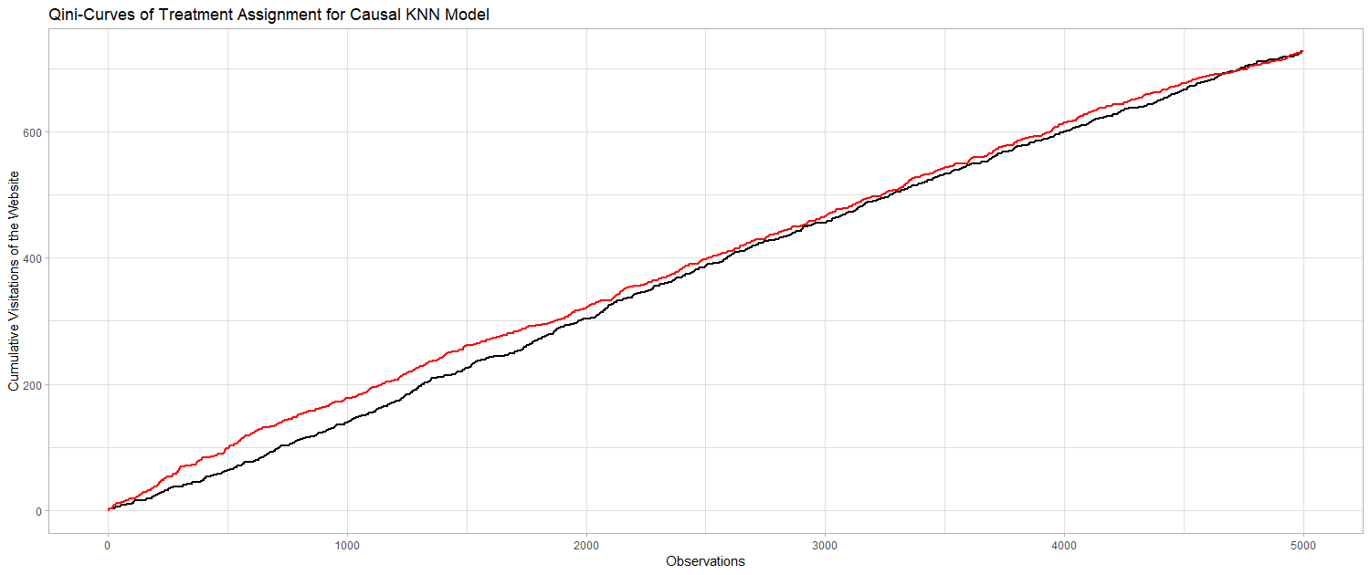
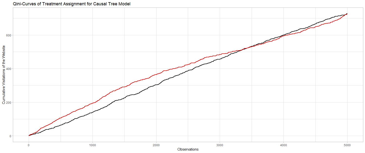
Qini Curves for evaluation of the causal KNN model
The Gini-Coefficient is a widely used metric to compare the fit of different modeling approaches on a particular data set. The metric is intuitive and applicable, since it provides a single value for the evaluation. The value of the Gini-Coefficient is defined between 0 and 1, where 1 represents a perfect model and 0 indicates a fit that is not performing any better than a random ranking of customers. Devriendt et al. (2018) state that the Gini-Coefficient, however, is not readily applicable in uplift modeling context, since for every class we have individuals from the treatment and the control group. Therefore, in this context, the so called “Qini-Coefficient” is preferred. The Qini-Coefficient is mathematically equal to the difference of the Gini-Curve for the treatment group and the control group. The Qini-Coefficient provides an opportunity to evaluate uplift models according to the treatment effect estmations. Since the Qini is a common indicator for the quality of uplift models, it is used here to evaluate the Causal KNN model results. Based on the calculated uplift factors for every individual, one could target only those individuals with the highest uplift, i.e. the highest probability of visiting the website after receiving an email. Treatment assignment based on the uplift values can be compared to the random assignment, where every individual gets a treatment with a probability of 2/3. Finally, one can look at the cumulative visits for the targeted customers. If the targeting of customers with a higher uplift also corresponds to a higher chance of visit, the curve of the Causal KNN predictions must be above the curve of the randomized predictions. We can use the same procedure to evaluate the predictions of the Causal Tree Model. The following to graphs are illustrating the desired result. If we first target the customers we identified using the two model approaches, we will gain more desired outcomes (i.e. visits) than for the randomized targeting.
AUUC
The AUUC is a common measure for model evaluation. This measure is defined by the area under the uplift curve. We can compare the resulting uplift curves to the optimal curve. Therefore it has strong relations to the Qini-Curve, but this measure does not take the incremental effect of random targeting into account. The following table contains measures to compare the two applied uplift modeling approaches.
| Model | MSE | AUUC |
|---|---|---|
| Causal KNN (K = 450) | 0.5508 | 0.34 |
| Causal Tree | 0.5321 | 0.36 |
When comparing both, the causal KNN and the causal tree model, it can be observed that the causal tree performs better than the Causal KNN model. This holds true for evaluating both models in terms of the MSE as well as for the area under the uplift curves (AUUC).
Conclusion
In this blogpost, we presented a method for estimating the conditional average treatment effect on an individual basis. This approach is called causal KNN. The causal KNN algorithm was implemented in R and applied to a real world data set from a randomized E-Mail marketing campaign. Furthermore, the Transformed Outcome was introduced, which represents the value of the “true” CATE in expectation, if several required assumptions to the data are fulfilled. The Transformed Outcome approach could be used for finding the optimal k value for the causal KNN model and also for the parameter tuning of other uplift modelling techniques. We trained a causal tree model to compare the results of our causal KNN estimations. The Transformed Outcome allowed for an evaluation of uplift models in terms of the MSE. Here, the causal tree performed better than the causal KNN model in terms of the MSE and the AUUC. Therefore, the causal KNN approach is a simple algorithm that delivers estimations of the CATE in uplift applications. However, the accuracy of the estimations is worse than those of comparable uplift models.
Code distribution
The full source Code can be found here: https://github.com/mkrcke/APA
References
Devriendt, F., Moldovan, D., & Verbeke, W. (2018). A literature survey and experimental evaluation of the state-of-the-art in uplift modeling: A stepping stone toward the development of prescriptive analytics. Big data, 6(1), 13-41.
Gutierrez, P., & Gerardy, J. Y. (2017, July). Causal inference and uplift modelling: A review of the literature. In International Conference on Predictive Applications and APIs (pp. 1-13).
Pearl, J. (2009). Causal inference in statistics: An overview. Statistics surveys, 3, 96-146.
Zhou, X., & Kosorok, M. R. (2017). Causal nearest neighbor rules for optimal treatment regimes. arXiv preprint arXiv:1711.08451.
Dudik, M., Langford, J., & Li, L. (2011). Doubly robust policy evaluation and learning. arXiv preprint arXiv:1103.4601.
Angrist, J. D. (2016). Treatment effect. The new Palgrave dictionary of economics, 1-8.
Jaskowski, M., & Jaroszewicz, S. (2012, June). Uplift modeling for clinical trial data. In ICML Workshop on Clinical Data Analysis.
Gubela, R. M., Lessmann, S., Haupt, J., Baumann, A., Radmer, T., & Gebert, F. (2017). Revenue Uplift Modeling.
Lo, V. S. (2002). The true lift model: a novel data mining approach to response modeling in database marketing. ACM SIGKDD Explorations Newsletter, 4(2), 78-86.
Athey, S., & Imbens, G. (2016). Recursive partitioning for heterogeneous causal effects. Proceedings of the National Academy of Sciences, 113(27), 7353-7360.
Coussement, K., Harrigan, P., & Benoit, D. F. (2015). Improving direct mail targeting through customer response modeling. Expert Systems with Applications, 42(22), 8403-8412.
Hitsch, G. J., & Misra, S. (2018). Heterogeneous treatment effects and optimal targeting policy evaluation. Available at SSRN 3111957.
Ascarza, E., Fader, P. S., & Hardie, B. G. (2017). Marketing models for the customer-centric firm. In Handbook of marketing decision models (pp. 297-329). Springer, Cham.
Paul R. Rosenbaum; Donald B. Rubin, The Central Role of the Propensity Score in Observational Studies for Causal Effects, Biometrika, Vol. 70, No. 1. (Apr., 1983), pp. 41-55.
Rzepakowski, P., & Jaroszewicz, S. (2012). Uplift modeling in direct marketing. Journal of Telecommunications and Information Technology, 43-50.
Athey, S., & Imbens, G. W. (2015). Machine learning methods for estimating heterogeneous causal effects. stat, 1050(5), 1-26.
Powers, S., Qian, J., Jung, K., Schuler, A., Shah, N. H., Hastie, T., & Tibshirani, R. (2017). Some methods for heterogeneous treatment effect estimation in high-dimensions. arXiv preprint arXiv:1707.00102.
Breiman, L. (1996). Bagging predictors. Machine learning, 24(2), 123-140.
Package References
H. Wickham. ggplot2: Elegant Graphics for Data Analysis. Springer-Verlag New York, 2016.
Hadley Wickham, Jim Hester and Romain Francois (2018). readr: Read Rectangular Text Data. R package version 1.3.0. https://CRAN.R-project.org/package=readr
Bischl B, Lang M, Kotthoff L, Schiffner J, Richter J, Studerus E, Casalicchio G, Jones Z (2016). mlr: Machine Learning in R. Journal of Machine Learning Research, 17(170), 1-5. <URL: http://jmlr.org/papers/v17/15-066.html>
Alina Beygelzimer, Sham Kakadet, John Langford, Sunil Arya, David Mount and Shengqiao Li (2019). FNN: Fast Nearest Neighbor Search Algorithms and Applications. R package version 1.1.3. https://CRAN.R-project.org/package=FNN
Hadley Wickham, Jim Hester and Winston Chang (2019). devtools: Tools to Make Developing R Packages Easier. R package version 2.0.2. https://CRAN.R-project.org/package=devtools
Susan Athey, Guido Imbens and Yanyang Kong (2016). causalTree: Recursive Partitioning Causal Trees. R package version 0.0.